Fire Monitoring Handbook

National Park Service

U.S. Department of the Interior

National Park Service

U.S. Department of the Interior

Fire Management Program Center

National Interagency Fire Center

Fire Monitoring Handbook

Preface i

3

Abstract

Fire is a powerful and enduring force that has had, and

The levels are cumulative, requiring users to include all

will continue to have, a profound influence on

levels below the highest specified.

National Park Service (NPS) lands. Fire management

decisions within the National Park Service require

The standards outlined in this handbook require moni-

information on fire behavior and on the effects of fire

toring at all four levels for prescribed fires. For levels 1

on park resources. With good reason, the public is

to 3, the handbook describes Recommended Standard

holding park management increasingly accountable,

variables, including fire conditions and vegetation

especially in the area of fire management. Federal and

parameters. Procedures and recommended frequencies

state agencies are instituting progressively more strin-

for monitoring and analysis are also specified.

gent guidelines for burning, monitoring, and evalua-

Depending on a park’s management objectives, a park

tion. The impetus behind these guidelines and the

may need a specific monitoring design beyond or

purpose of this handbook are to ensure that manage-

instead of the design covered in this handbook. Refer-

ment objectives are being met, to provide guidance

ences to different monitoring procedures are provided

that can prevent fire management problems from

in the appendices.

developing, to limit possible legal actions against the

agency, and to ensure that all parks collect at least the

A standardized system to cover the wide diversity of

minimum information deemed necessary to evaluate

areas within the National Park Service will need fine-

their fire management programs.

tuning from park to park. To facilitate this, each park

will receive oversight and review for its monitoring

There are many benefits to establishing these standard-

program from its regional fire monitoring program

ized data collection procedures. Uniformly-gathered

manager, and refinements to this Fire Monitoring

data will facilitate information exchange among parks

Handbook will be made as necessary. Until a subse-

and provide historical program documentation and

quent revision of this handbook is published, these

databases useful for refinements of the parks’ fire

refinements will be made available on the Internet at

management programs. In addition, standard proce-

<www.nps.gov/fire/fire/fir_eco_monitoring.html>

dures will enable fire monitors to move to or assist

Also at this website is information on how parks

other parks without additional training.

are using their data and how to download the

associated software.

The fire monitoring program described in this Fire

Monitoring Handbook (FMH) allows the National

USDI National Park Service. 2003. Fire Moni-

Park Service to document basic information, to detect

toring Handbook. Boise (ID): Fire Manage-

trends, and to ensure that each park meets its fire and

ment Program Center, National Interagency

resource management objectives. From identified

Fire Center. 274p.

trends, park staff can articulate concerns, develop

hypotheses, and identify specific research studies to

develop solutions to problems.

This handbook is intended to facilitate and standardize

monitoring for National Park Service units that are

subject to burning by wildland or prescribed fire. This

K

eywords: Fire Behavior, Fire Monitoring, Adaptive

handbook defines and establishes levels of monitoring

Management, Vegetation Monitoring, Sampling,

activity relative to fire and resource management

Sampling Design, Objective Development, Wildland

objectives and fire management strategies. At each suc-

Fire, Prescribed Fire.

cessive level, monitoring is more extensive and com-

plex. level 1 covers environmental monitoring, and

levels 2, 3, and 4 call for monitoring of fire conditions,

Printed on Recycled Paper

short-term change, and long-term change, respectively.

Fire Monitoring Handbook ii

Task Force Co

nsultants and Reviewers

ask Force Consultants and Reviewers

Acknowledgments

Many have worked toward the development of this handbook. While we cannot possibly acknowledge all contrib-

utors, including all the people who used this methodology and provided us with comments, we would like to rec-

ognize individuals who were critical to this effort.

Fire Monitoring Steering Committee, 1977

Stephen J. Botti (Task Force Chairperson), National Park Service,

National Interagency Fire Center

Craig Allen, US Geological Survey, Biological Resources Division, Dan O’Brien, National Park Service, Intermountain Regional Office,

Bandelier National Monument retired

Elizabeth Anderson, National Park Service, Intermountain Regional Rebecca Power (Representative, Region 3 Fire Monitoring Task

Office, retired Force), US Fish and Wildlife Service, Necedah National Wildlife Refuge

MaryBeth Keifer, Sequoia and Kings Canyon National Parks Doug Wallner, National Park Service, Philadelphia Support Office

Task Force Consultants and Reviewers

Jonathan Arnold

Lassen Volcanic National Park

Henry Bastian, Zion National Park

Pam Benjamin, National Park Service, Intermountain Regional Office

Ed Berg, US Fish and Wildlife Service, Kenai National Wildlife Refuge

Frank Boden, Bureau of Indian Affairs, retired

Beth Buchanan, Daniel Boone National Forest

Dan Buckley,Yosemite National Park

Gary Davis, Channel Islands National Park

John Dennis, National Park Service, Natural Resource, Information Division

Robert Dellinger, Great Smoky Mountains National Park

Dennis Divoky, Glacier National Park

Gregory Eckert, National Park Service,

Biological Resource Management Division

Steve Fancy, National Park Service,

Natural Resource, Information Division

Patti Haggarty, Corvallis Forest Science Laboratory

Walter Herzog, Bureau of Land Management,

Redding Resource Area

Laura Hudson, National Park Service, Intermountain Regional Office

Roger Hungerford, USDA Forest Service

Intermountain Research Station, retired

Ben Jacobs, Point Reyes National Seashore

Evelyn Klein, Lyndon B. Johnson National Historical Park, retired

Mary Kwart, US Fish and Wildlife Service,

Tetlin National Wildlife Refuge

Bill Leenhouts, Fish and Wildlife Service,

National Interagency Fire Center

Michael Loik, University of California

Mack McFarland, Grand Teton National Park

Melanie Miller, Bureau of Land Management, National Interagency Fire Center

Wesley Newton, US Geological Survey Biological Resources,

Division Northern Prairie Wildlife Research Center

Howard T. Nichols, Pacific West Regional Office

Larry Nickey, Olympic National Park

Tonja Opperman, Bitterroot National Forest

William Patterson III, University of Massachusetts

Arnie Peterson, Lassen Volcanic National Park

Nathan Rudd, The Nature Conservancy, Oregon Field Office

Kevin Ryan, Intermountain Fire Sciences Lab

Kathy Schon, Saguaro National Park

Tim Sexton, National Park Service National Interagency Fire Center

Carolyn Hull Sieg, Rocky Mountain Research Station

Geoffrey Smith

Apostle Islands National Lakeshore

Tom Stohlgren, US Geological Survey Biological Resources Division, Colorado

State University

Tim Stubbs, Carlsbad Caverns National Park

Gary Swanson, US Fish and Wildlife Service,

Sherburne National Wildlife Refuge

Charisse Sydoriak, Bureau of Land Management

Alan Taylor

Pennsylvania State University

Lisa Thomas, Wilson’s Creek National Battlefield

Laura Trader, Bandelier National Monument

Jan Van Wagtendonk, US Geological Survey

Biological Resources Division, Yosemite Field Station

C. Phillip Weatherspoon, US Forest Service

Pacific Southwest Forest and Range Experiment Station

Meredith Weltmer, US Fish and Wildlife Service, Region 3

John Willoughby, Bureau of Land Management, California State Office

Preface iii

Steering Committee Support Staff:

Rewrite Committee

Paul Reeberg (Coordinator, Content Editor) Eric Allen, Jewel Cave National Monument

National Park Service, Pacific West Regional Office

MaryBeth Keifer, Sequoia and Kings Canyon National Parks Richard Bahr, National Interagency Fire Center

Elizabeth Anderson, National Park Service, Intermountain Regional Tony LaBanca, California Department of Fish and Game, Northern

Office, retired California-North Coast Region

Stassia Samuels, Redwood National and State Parks Rick Anderson, Archbold Biological Station

Jeanne E. Taylor, Golden Gate National Recreation Area, retired John Segar, Boise National Forest

Dale Haskamp, Redwood National and State Parks, retired

Data Entry and Processing Software

Walter M. Sydoriak (Developer), Bandelier National Monument

Tim Sexton (Coordinator), National Interagency Fire Center

Editorial Review

Kathy Rehm Switky, Menlo Park, CA

Formatting

Paul Reeberg and Brenda Kauffman

National Park Service, Pacific West Regional Office

Design and Illustration

Eugene Fleming

National Park Service, Pacific West Regional Office

Cover Photography

Fire on the Ridge: © Richard Blair, www.richardblair.com

Shoot emerging from pine needles: © Michael S. Quinton, National

Geographic Society

Fire Monitoring Handbook iv

- - - - - - - - - - - - - -

Contents

Abstract - - - - - - - - - - - - - - - - - - - - - - - - ii

Acknowledgments - -- - - - -- - - - -- - - - - - - - - - - -- - - - - - - - iii

Use of this Handbook -- - - - -- - - - -- - - - - - - - - - - -- - - - - - - - ix

Symbols Used in this Handbook - - - -- - - - - - - - - - - -- - - - - - - - x

Chapter 1 Introduction - - - - - - - - - - - - - - - - - - - - - - - - - 1

Fire Monitoring Policy - -- - - - -- - - - - - - - - - - -- - - - - - - - 1

Recommended Standards -- - - - -- - - - - - - - - - - -- - - - - - - - 2

Some Cautions -- - - - -- - - - -- - - - - - - - - - - -- - - - - - - - 2

Fire Management Strategies - - - -- - - - - - - - - - - -- - - - - - - - 3

Program Responsibilities of NPS Personnel - - - - - - - - -- - - - - - - - 4

Fire Monitoring Levels - -- - - - -- - - - - - - - - - - -- - - - - - - - 4

Chapter 2 Environmental & Fire Observation - -- - - - - - - - - - - -- - - - - - - - 7

Monitoring Level 1: Environmental Monitoring - - - - - - - -- - - - - - - - 7

Monitoring Schedule - - -- - - - -- - - - - - - - - - - -- - - - - - - - 7

Procedures and Techniques-- - - - -- - - - - - - - - - - -- - - - - - - - 7

Monitoring Level 2: Fire Observation- - - - - - - - - - - - - - - - - 9- - - - -

Reconnaissance Monitoring - -- - - - -- - - - - - - - - - - -- - - - - - - - 9

Monitoring Schedule - - -- - - - -- - - - - - - - - - - -- - - - - - - - 9

Procedures and Techniques-- - - - -- - - - - - - - - - - -- - - - - - - - 9

Fire Conditions Monitoring - -- - - - -- - - - - - - - - - - -- - - - - - - -11

Monitoring Schedule - - -- - - - -- - - - - - - - - - - -- - - - - - - -11

Procedures and Techniques-- - - - -- - - - - - - - - - - -- - - - - - - -11

Postburn Report -- - - - -- - - - -- - - - - - - - - - - -- - - - - - - -15

Chapter 3 Developing Objectives -- - - - -- - - - -- - - - - - - - - - - -- - - - - - - -19

Objectives - - - - - - - - - - - - - - - - - - - - - - - - - - - - -- - - - - - - - 20

Management Objectives - -- - - - -- - - - - - - - - - - -- - - - - - - -20

Monitoring Objectives - -- - - - -- - - - - - - - - - - -- - - - - - - -23

Objective Variables - -- - - - -- - - - -- - - - - - - - - - - -- - - - - - - -29

Comparing Vegetation Attributes - -- - - - - - - - - - - -- - - - - - - -30

Point Intercept Method - -- - - - -- - - - - - - - - - - -- - - - - - - -31

Other Methods -- - - - -- - - - -- - - - - - - - - - - -- - - - - - - -32

Chapter 4 Monitoring Program Design - -- - - - -- - - - - - - - - - - -- - - - - - - -33

Monitoring Types - - -- - - - -- - - - -- - - - - - - - - - - -- - - - - - - -34

Defining Monitoring Types - - - -- - - - - - - - - - - -- - - - - - - -34

Variables - - - - - - - - - - - - - - - - - - - - - - - -41

Level 3 and 4 Variables -- - - - -- - - - - - - - - - - -- - - - - - - -41

RS Variables - -- - - - -- - - - -- - - - - - - - - - - -- - - - - - - -41

Sampling Design - - -- - - - -- - - - -- - - - - - - - - - - -- - - - - - - -43

Pilot Sampling -- - - - -- - - - -- - - - - - - - - - - -- - - - - - - -43

Deviations or Additional Protocols - - - - - - - - - - - - - - - -47- - - - -

Considerations Prior to Further Plot Installation- - - - - - -- - - - - - - -48

Sampling Design Alternatives - - -- - - - - - - - - - - -- - - - - - - -48

Calculating Minimum Sample Size - - - - - - - - - - - - - - - -49- - - - -

Monitoring Design Problems - - - -- - - - - - - - - - - -- - - - - - - -50

Control Plots - -- - - - -- - - - -- - - - - - - - - - - -- - - - - - - -52

Dealing with Burning Problems - -- - - - - - - - - - - -- - - - - - - -53

Chapter 5 Vegetation Monitoring Protocols - - -- - - - - - - - - - - -- - - - - - - -55

Methodology Changes - - -- - - - -- - - - - - - - - - - -- - - - - - - -55

Preface v

- - - -

Monitoring Schedule - - -- - - - -- - - - -- - - - - - - - - - - - - - - 55

Generating Monitoring Plot Locations -- - - - -- - - - - - - - - - - - - - - 59

Creating Equal Portions for Initial Plot Installation - - - - - - - - - - - - 60

Creating n Equal Portions Where Plots Already Exist - - - - - - - - - - - 60

Randomly Assigning Plot Location Points - -- - - - - - - - - - - - - - - 60

Plot Location -- - - - -- - - - -- - - - -- - - - -- - - - - - - - - - - - - - - 62

Step 1: Field Locating PLPs - - -- - - - -- - - - - - - - - - - - - - - 62

Laying Out and Installing Monitoring Plots - - -- - - - - - - - - - - - - - - 64

Grassland and Brush Plots - - - -- - - - -- - - - - - - - - - - - - - - 64

Forest Plots- - -- - - - -- - - - -- - - - -- - - - - - - - - - - - - - - 67

Labeling Monitoring Plot Stakes - - - -- - - - -- - - - - - - - - - - - - - - 70

Photographing the Plot - - - -- - - - -- - - - -- - - - - - - - - - - - - - - 71

Grassland and Brush Plots - - - -- - - - -- - - - - - - - - - - - - - - 71

Forest Plots- - -- - - - -- - - - -- - - - -- - - - - - - - - - - - - - - 71

RS Procedures- - - - - - - - - - - - - - - - - -

Step 2: Assessing Plot Acceptability and Marking Plot Origin - - - - - - - - 62

- - - - - - - - - - - - - - 71

Equipment and Film- - -- - - - -- - - - -- - - - - - - - - - - - - - - 72

Field Mapping the Monitoring Plot- - -- - - - -- - - - - - - - - - - - - - - 75

Complete Plot Location Data Sheet -- - - - -- - - - - - - - - - - - - - - 75

Monitoring Vegetation Characteristics -- - - - -- - - - - - - - - - - - - - - 80

All Plot Types - - - - - - - - - - - - - - - - -- - - - - - - - - - - - - - 80

Herbaceous and Shrub Layers - - -- - - - -- - - - - - - - - - - - - - - 80

Brush and Forest Plots - -- - - - -- - - - -- - - - - - - - - - - - - - - 87

Monitoring Overstory Trees - -- - - - -- - - - -- - - - - - - - - - - - - - - 91

Tag and Measure All Overstory Trees - - - -- - - - - - - - - - - - - - - 91

Optional Monitoring Procedures - -- - - - -- - - - - - - - - - - - - - - 93

Monitoring Pole-size Trees - -- - - - -- - - - -- - - - - - - - - - - - - - 100

Measure Density and DBH of Pole-size Trees - - - - - - - - - - - - - 100

Optional Monitoring Procedures - -- - - - -- - - - - - - - - - - - - - 100

Monitoring Seedling Trees- - -- - - - -- - - - -- - - - - - - - - - - - - - 102

Count Seedling Trees to Obtain Species Density - - - - - - - - - - - - - 102

Optional Monitoring Procedures - -- - - - -- - - - - - - - - - - - - - 102

Monitoring Dead and Downed Fuel Load - - -- - - - - - - - - - - - - - 103

RS Procedures- - - - - - - - - - - - - - - - - - - - - - - - - - - - - - - 103

Deal with Sampling Problems - - -- - - - -- - - - - - - - - - - - - - 105

Monitoring Fire Weather and Behavior Characteristics - - - - - - - - - - 106

Rate of Spread - - - - - - - - - - - - - - - - - - - - - - - - - - - - - - 106

Flame Length and Depth -- - - - -- - - - -- - - - - - - - - - - - - - 106

Monitoring Immediate Postburn Vegetation & Fuel Characteristics - - - - 108

Grassland and Brush Plots - - - -- - - - -- - - - - - - - - - - - - - 108

Forest Plots - - - - - - - - - - - - - - - - - - - - - - - - - - - 108

Monitor Postburn Conditions - - -- - - - -- - - - - - - - - - - - - - 108

Optional Monitoring Procedures - -- - - - -- - - - - - - - - - - - - - 111

File Maintenance & Data Storage - - -- - - - -- - - - - - - - - - - - - - 112

Plot Tracking - - - - - - - - - - - - - - - - - - - - - - - - - - - 112

Monitoring Type Folders -- - - - -- - - - -- - - - - - - - - - - - - - 112

Monitoring Plot Folders -- - - - -- - - - -- - - - - - - - - - - - - - 112

Slide—Photo Storage - -- - - - -- - - - -- - - - - - - - - - - - - - 112

Field Packets - - - - - - - - - - - - - - - - - - - - - - - - - - - - - - - 112

Data Processing and Storage - - - -- - - - -- - - - - - - - - - - - - - 113

Ensuring Data Quality - - - -- - - - -- - - - -- - - - - - - - - - - - - - 114

Quality Checks When Remeasuring Plots - -- - - - - - - - - - - - - - 114

Quality Checks in the Field - - - -- - - - -- - - - - - - - - - - - - - 115

Fire Monitoring Handbook vi

- - - - - - - -

Quality Checks in the Office - - - -- - - - - - - - - - - -- - - - - - - 115

Quality Checks for Data Entry- - -- - - - - - - - - - - -- - - - - - - 116

Chapter 6 Data Analysis and Evaluation- -- - - - -- - - - - - - - - - - -- - - - - - - 119

Level 3: Short-term Change- - - - -- - - - - - - - - - - -- - - - - - - 119

Level 4: Long-term Change- - - - -- - - - - - - - - - - -- - - - - - - 119

The Analysis Process -- - - - -- - - - -- - - - - - - - - - - -- - - - - - - 121

Documentation -- - - - - - - - - - - - - - - - - - - - - - - - - - - - - 121

Examining the Raw Data - - - -- - - - - - - - - - - -- - - - - - - 121

Summarizing the Data - -- - - - -- - - - - - - - - - - -- - - - - - - 122

Recalculating the Minimum Sample Size - - - - - - - - - -- - - - - - - 124

Additional Statistical Concepts - - - - -- - - - - - - - - - - -- - - - - - - 126

Hypothesis Tests - - - -- - - - - - - -- - - - - - - - -- - - - - - - 126

Interpreting Results of Hypothesis Tests - - - - - - - - - -- - - - - - - 128

- - - - -The Evaluation Process - - - -- - - - - - - - - - - - - - - - - - - 130

Evaluating Achievement of Management Objectives - - - - -- - - - - - - 130

Evaluating Monitoring Program or Management Actions - - -- - - - - - - 131

Disseminating Results - -- - - - -- - - - - - - - - - - -- - - - - - - 134

Reviewing the Monitoring Program - - - - - - - - - - - - - - - 135- - - - -

Appendix A Monitoring Data Sheets -- - - - -- - - - -- - - - - - - - - - - -- - - - - - - 137

Appendix B Random Number Generators - -- - - - - - - - - - - - - - - - - - - 189- - - - -

Using a Table -- - - - -- - - - -- - - - - - - - - - - -- - - - - - - 189

Using Spreadsheet Programs to Generate Random Numbers - -- - - - - - -

Tools and Supplies - - - -- - - - - - - - - - - - - - - - - - - 194

191

Appendix C Field Aids -- - - - - - - - - - - - - - - - - - - - - - - - - - - - - - - 193

Collecting & Processing Voucher Specimens - - - - - - - - -- - - - - - - 193

Collecting - - -- - - - -- - - - -- - - - - - - - - - - -- - - - - - - 193

- - - - -

Pressing and Drying - - -- - - - - - - -- - - - - - - - -- - - - - - - 195

Mounting, Labeling and Storing - -- - - - - - - - - - - -- - - - - - - 197

Identifying Dead & Dormant Plants - -- - - - - - - - - - - -- - - - - - - 199

Resources - - -- - - - -- - - - -- - - - - - - - - - - -- - - - - - - 199

Observations - -- - - - -- - - - -- - - - - - - - - - - -- - - - - - - 199

Navigation Aids - - -- - - - -- - - - -- - - - - - - - - - - -- - - - - - - 201

Compass - - - -- - - - -- - - - -- - - - - - - - - - - -- - - - - - - 201

Using a Compass in Conjunction with a Map - - - - - - - -- - - - - - - 201

Clinometer - - -- - - - -- - - - -- - - - - - - - - - - -- - - - - - - 202

Determining Distances in the Field -- - - - - - - - - - - -- - - - - - - 203

Some Basic Map Techniques - - - -- - - - - - - - - - - -- - - - - - - 204

Global Positioning System Information - - - - - - - - - - -- - - - - - - 205

Basic Photography Guidelines -- - - - -- - - - - - - - - - - -- - - - - - - 207

Conversion Tables - -- - - - -- - - - -- - - - - - - - - - - -- - - - - - - 209

Appendix D Data Analysis Formulae -- - - - -- - - - -- - - - - - - - - - - -- - - - - - - 213

Cover - - - - - - - - - - - - - - - - - - - - - - - - - - - - - - - - - - - 213

Tree, Herb, and Shrub Density - -- - - - - - - - - - - -- - - - - - - 213

Fuel Load - - -- - - - -- - - - -- - - - - - - - - - - -- - - - - - - 214

Data Analysis Calculations - - - -- - - - - - - - - - - -- - - - - - - 216

Appendix E Equipment Checklist - - -- - - - -- - - - -- - - - - - - - - - - -- - - - - - - 221

Locating, Marking, and Installing a Monitoring Plot - - - - -- - - - - - - 221

Monitoring Forest Plots - -- - - - -- - - - - - - - - - - -- - - - - - - 221

Monitoring Brush and Grassland Plots - - - - - - - - - -- - - - - - - 222

Monitoring During a Prescribed Fire - - - - - - - - - - -- - - - - - - 222

Monitoring During a Wildland Fire - - - - - - - - - - -- - - - - - - 223

Optional Equipment - - -- - - - -- - - - - - - - - - - -- - - - - - - 224

Appendix F Monitoring Plan Outline -- - - - -- - - - -- - - - - - - - - - - -- - - - - - - 225

Preface vii

0

Introduction (General) - -- - - - -- - - - -- - - - - - - - - - - - - - 225

Description of Ecological Model - -- - - - -- - - - - - - - - - - - - - 225

Management Objective(s) -- - - - -- - - - -- - - - - - - - - - - - - - 225

Monitoring Design - - - -- - - - -- - - - -- - - - - - - - - - - - - - 225

Appendix G Additional Reading - - - -- - - - -- - - - -- - - - -- - - - - - - - - - - - - - 229

References for Nonstandard Variables -- - - - -- - - - - - - - - - - - - - 229

General - - - -- - - - -- - - - -- - - - -- - - - - - - - - - - - - - 229

Fire Conditions and Observations -- - - - -- - - - - - - - - - - - - - 230

Air, Soil and Water - - -- - - - -- - - - -- - - - - - - - - - - - - - 231

Forest Pests (Mistletoe, Fungi, and Insects) - -- - - - - - - - - - - - - - 232

Amphibians and Reptiles -- - - - -- - - - -- - - - - - - - - - - - - - 233

Birds -- - - - - - - - - - - - - - - - - - - - - - - - - - - - - - - - - - 234

Mammals - - - - - - - - - - - - - - - - - - - - - - - - - - - - - - - - 236

Vegetation - - -- - - - -- - - - -- - - - -- - - - - - - - - - - - - - 237

Fuels -- - - - - - - - - - - - - - - - - - - - - - - - - - - - - - - - - - 237

Adaptive Management - -- - - - -- - - - -- - - - - - - - - - - - - - 239

Vegetative Keys - - - - - - - - - - - - - - - - - - - - - - - - - - - - - - - - 240

Glossary of Terms -- - - - - - - - - - - -- - - - - - - - -- - - - - -- - - - -- - - - - - - - - - - - - - 247

References - - - - - - - - - - - - - - - - - - - - - - - - 259- - - - - - - - - - - - - - - - - - - - - - - - - - - -

Cited References - - - -- - - - -- - - - -- - - - - - - - - - - - - - 259

Additional References - -- - - - -- - - - -- - - - - - - - - - - - - - 261

Index - - - -- - - - - - - -- - - - - - - - -- - - - - - - - -- - - - - -- - - - -- - - - - - - - - - - - - - 263

0

Fire Monitoring Handbook viii

Use of this Handbook

The handbook presents detailed instructions for fire

monitoring in a variety of situations. The instructions

are organized around the management strategies fre-

quently used to meet specific objectives.

Each chapter covers a different aspect of fire effects

monitoring. You will find an overview of each area,

and the functions within that area, at the beginning of

each chapter.

Chapter 1: Introduction—an overview of the entire

National Park Service Fire Monitoring program.

Chapter 2: Environmental and Fire Observation—a

detailed discussion of the monitoring schedule and

procedures involved with monitoring levels 1 (environ-

mental) and 2 (fire observation).

Chapter 3: Developing Objectives—development of

objectives and the basic management decisions neces-

sary to design a monitoring program. This basic design

is expanded upon in chapter four.

Chapter 4: Monitoring Program Design—detailed

instructions for designing a monitoring program for

short-term and long-term change, randomizing moni-

toring plots, and choosing monitoring variables.

Chapter 5: Vegetation Monitoring Protocols—

detailed procedures for reading plots designed to mon-

itor prescribed fires (at levels 3 and 4) for forest, grass-

land and brush plot types.

Chapter 6: Data Analysis and Evaluation—guidance

for data analysis and program evaluation.

Appendices: data record forms, random number

tables, aids for data collection, useful equations, refer-

ences describing methods not covered in this hand-

book, and handbook references.

This handbook is designed to be placed in a binder so

that you can remove individual chapters and appendi-

ces. You can detach the instructions for the applicable

monitoring level required for a fire from the binder

and carry them into the field for easy reference.

Field Handbook

If you need a small portable version of this

handbook, use a copy machine to create a ¼ size

version of the pages you will need in the field (e.g.,

Chapter 5, Appendix C).

Preface ix

Symbols Used in this Handbook

Note: Refer to the Index for the location of the fol-

lowing symbols within this handbook.

Reminder

This symbol indicates information that

you won’t want to forget!

Tip from the Field

This symbol indicates advice from expe-

rienced field folks. Additional field tips

may be found in Elzinga and others

(1998), pages 190–1 (marking the plot),

192–6 (field equipment) and page 406

(general field tips).

Warning

This symbol denotes potentially hazard-

ous or incorrect behavior. It is also used

to indicate protocol changes since the

last revision of this Fire Monitoring

Handbook (NPS 1992).

Fire Monitoring Handbook x

Introduction

1

Introduction

“Not everything that can be counted counts, and not everything that counts can be counted.”

—Albert Einstein

Fire is a powerful and enduring force that has had,

and will continue to have, a profound influence on

National Park Service (NPS) lands. Restoring and

maintaining this natural process are both impor-

tant management goals for many NPS areas. There-

fore, information about the use and effects of

prescribed fire on park resources is critical to

sound, scientifically-based management decisions.

Using results from a high quality monitoring pro-

gram to evaluate your prescribed fire management

program is the key to successful adaptive manage-

ment. By using monitoring results to determine

whether you are meeting your management objec-

tives, you can verify that the program is on track,

or conversely, gather clues about what may not be

working so that you can make appropriate

changes.

This fire monitoring program allows the National

Park Service to document basic information, to

detect trends, and to ensure that parks meet their

fire and resource management objectives. From

identified trends, park staff can articulate concerns,

develop hypotheses, and identify specific research

projects to develop solutions to problems. The

goals of the program described here are to:

Document basic information for all wildland

fires, regardless of management strategy

Document fire behavior to allow managers to

take appropriate action on all fires that either:

• have the potential to threaten resource values

• are being managed under specific constraints,

such as a prescribed fire or fire use

Document and analyze both short-term and

long-term prescribed fire effects on vegetation

Establish a recommended standard for data col-

lection and analysis techniques to facilitate the

sharing of monitoring data

Follow trends in plant communities where fire

effects literature exists, or research has been

conducted

Identify areas where additional research is needed

This Fire Monitoring Handbook (FMH) describes

the procedures for this program in National Park

Service units.

FIRE MONITORING POLICY

Staff in individual parks document the rationale,

purpose, and justification of their fire management

programs in their Natural Resource Management

Plans and Fire Management Plans. Director’s

Order #18: Wildland Fire Management (DO-18)

(USDI National Park Service 1998) outlines

National Park Service fire management policies,

which are expanded upon in Reference Manual-18:

Wildland Fire Management (RM-18) (USDI

National Park Service 2001a).

Provisions of NEPA

The National Environmental Policy Act (42 USC

4321–4347), NEPA (1969), mandates that monitor-

ing and evaluation be conducted to mitigate human

actions that alter landscapes or environments. The

Code of Federal Regulations (CFR) provides the

following legal directives:

40 CFR Sec. 1505.03

“Agencies may provide for monitoring to

assure that their decisions are carried out and

should do so in important cases.”

40 CFR Sec. 1505.2(cl)

“A monitoring and enforcement program shall

be adopted and summarized when applicable

for any mitigation.”

DO-18: Wildland Fire Management

DO-18: Wildland Fire Management (USDI NPS

1998) directs managers to monitor all prescribed

and wildland fires. Monitoring directives (summa-

rized here from DO-18) are:

Fire effects monitoring must be done to evaluate

the degree to which objectives are accomplished

1

Long-term monitoring is required to document

that overall programmatic objectives are being met

and undesired effects are not occurring

Evaluation of fire effects data are the joint respon-

sibility of fire management and natural resource

management personnel

Neither DO-18 nor RM-18 describes how monitoring

is to be done. This handbook provides that guidance

by outlining standardized methods to be used through-

out the National Park Service for documenting, moni-

toring, and managing both wildland and prescribed

fires.

RECOMMENDED STANDARDS

This handbook outlines Recommended Standards

(RS) for fire monitoring within the National Park Ser-

vice. These standard techniques are mandatory for

Environmental (level 1) and Fire Observation

(level 2) monitoring. The techniques presented for

Short-term change (level 3) and Long-term change

(level 4) monitoring are confined to vegetation

monitoring, and will not answer all questions

about the effects of fire management programs on

park ecosystems. Many parks will require addi-

tional research programs to study specific issues

such as: postburn erosion, air and water quality,

wildlife, cultural resources, and the cumulative

effects of burning on a landscape scale. Parks are

encouraged to expand long-term monitoring to

include any additional physical or biotic ecosystem

elements important to management but not cov-

ered by these Recommended Standards.

Consult a regional fire monitoring coordinator, local

researcher, resource manager, and/or fire manager

before eliminating or using protocols other than

the Recommended Standards. For example, park

managers should not eliminate fuel transects in a

forest plot because they do not want to spend the

time monitoring them. However, if during the

pilot sampling period (see page 43) another sampling

method performs better statistically than a method

prescribed by this handbook, it is then recommended

that you substitute this other sampling method.

SOME CAUTIONS

Monitoring vs. Research

Monitoring (as defined in the Glossary) is always

driven by fire and resource management objectives,

and is part of the adaptive management cycle. As

part of this cycle, it is used to measure change over

time, and can therefore help evaluate progress

toward or success at meeting an objective. Monitor-

ing can also provide a basis for changing manage-

ment actions, if needed.

Research (as defined in the Glossary) is often

focused on identifying correlation of change with a

potential cause. Few monitoring projects can iden-

tify this correlation. As you move along the contin-

uum from monitoring to research, you gain

increased confidence as to the cause of a response,

often with an associated increase in study costs.

Because a monitoring program does not control for

potential causes, monitoring data should not be

mistaken for information on cause and effect. If

you need causality data for a management objec-

tive, you will need input from a statistician and/or

research scientist for a research study design.

A distinction has traditionally been made between

research and monitoring, but as monitoring programs

become better designed and statistically sound, this

distinction becomes more difficult to discern. A moni-

toring program without a well-defined objective is like

a research experiment without a hypothesis. Likewise,

statistically testing whether an objective has been met

in a monitoring program is very similar to hypothesis

testing in a research experiment. Knowing which sta-

tistical test is appropriate, along with the assumptions

made by a particular test, is critical in order to

avoid making false conclusions about the results.

Because statistical procedures can be complex, it is

recommended that you consult with a statistician

when performing such tests.

Control Plots

Install control plots (see Glossary, and page 52) when

it is critical to isolate the effects of fire from other

environmental or human influences, or to meet spe-

cific requirements, e.g., a prescribed fire plan. Control

plot sampling design will necessarily be specific to the

site and objective, and will require assistance from sub-

ject-matter experts.

Alternative Methods

If your management staff chooses objectives that

you cannot monitor using the protocols discussed

in this handbook, you will need to develop appro-

priate sampling methods. For example, objectives

FiFirree MMononititororiingng HaHandbndbookook 22

set at the landscape level (large forest gaps), or that

relate to animal populations would require additional

methods. Appendix G lists several monitoring refer-

ences for other sampling methods. Develop custom-

ized monitoring systems with the assistance of subject-

matter experts. Your regional fire monitoring coordi-

nator must review any alternative methodology.

Required Research

Park staff should have fire management program

objectives that are definable and measurable (see

page 20) and knowledge to reasonably predict fire

effects. If these criteria are not met, fire ecologists

should conduct research to determine the role of

fire in the park and develop prescriptions capable

of meeting park management objectives. The park

may need to delay implementation of its prescribed

fire management program until these issues are

resolved. Following this resolution, monitoring

must be initiated to assess the need for changes in

the program.

FIRE MANAGEMENT STRATEGIES

This handbook is organized around fire management

strategies that are directed by resource and fire man-

agement objectives. A Recommended Standard

monitoring level is given for each management

strategy. Table 1 outlines monitoring levels required

for wildland fire management strategies. The informa-

tion collected at each of these levels is the recom-

mended minimum; park staffs are encouraged to

collect additional information within their monitoring

programs as they see fit.

Suppression

Park managers often set fire suppression goals in

order to minimize negative consequences of wild-

land fires. A fire suppression operation will have

well-established and standardized monitoring needs

based on these goals. For most suppressed wildland

fires, monitoring means recording data on fire

cause and origin, discovery, size, cost, and location.

This is the reconnaissance portion of level 2 moni-

toring (fire observation; see page 9).

Monitoring the effect of suppressed wildland fires on

vegetation or other area-specific variables of special

concern may produce valuable information on fire

effects, identify significant threats to park resources, or

permit adjustments to appropriate suppression actions.

This information may drive the need for a rehabilita-

tion response to a wildland fire.

An additional caution here is that fire funds will not

pay for levels 3 and 4 monitoring of suppression

fires.

Wildland Fire Use

Fire management programs that focus on maintaining

natural conditions in native ecosystems generally need

different management strategies and have different

monitoring needs. These programs will meet the Rec-

ommended Standard by collecting the data needed to

complete Stage I of the Wildland Fire Implementation

Plan (see Glossary). This is Fire Observation level 2

monitoring, which includes reconnaissance (see page

9) and fire conditions (see page 11).

Table 1. Wildland fire management strategies and Recommended Standard (RS) monitoring levels.

Management Strategy RS Level

Suppression: All management actions are intended to extinguish or limit the growth of the

fire.

1. Environmental

2. Fire Observation

–Reconnaissance

Wildland Fire Use: Management allows a fire started by a natural source to burn as long as it

meets prescription standards.

1. Environmental

2. Fire Observation

–Reconnaissance

–Fire Conditions

Prescribed Fire: Management uses intentionally set fires as a management tool to meet

management objectives.

1. Environmental

2. Fire Observation

–Reconnaissance

–Fire Conditions

3. Short-term Change

4. Long-term Change

Chapter 1 n

nn

n Introduction 3

Prescribed Fire

Prescribed fire requires a much more complex moni-

toring system to document whether specific objec-

tives are accomplished with the application of fire.

The Recommended Standard here includes a hierar-

chy of monitoring levels from simple reconnais-

sance to the complex monitoring of prescriptions,

immediate postburn effects, and the long-term

changes in vegetation community structure and

succession. Measuring the effectiveness of pre-

scribed fire for natural ecosystem restoration may

take decades.

Managers can use research burns to expand their

knowledge of fire ecology. However, this handbook

does not cover the sampling design necessary for these

burns. Your regional fire ecologist can assist you with

this design.

PROGRAM RESPONSIBILITIES OF NPS

PERSONNEL

Implementation of this monitoring program

requires substantial knowledge. Park fire manage-

ment officers and natural resource managers must

understand ecological principles and basic statistics.

Park superintendents are responsible for implementing

and coordinating a park’s fire monitoring program.

They also may play active roles on program review

boards established to assess whether monitoring

objectives are being met, and whether information

gathered by a monitoring effort is addressing key park

issues.

Fire management personnel are responsible for

assuring the completion of environmental monitor-

ing (level 1) as part of the fire management plan

process, as well as daily observations and continual

field verification.

Fire management personnel are also responsible for

collecting fire observation monitoring data (level 2)

for each fire. These observations are needed as part of

the Initial Fire Assessment, which documents the deci-

sion process for the Recommended Response Action.

This then becomes Stage I in the Wildland Fire Imple-

mentation Plan for a “go” decision to elicit the appro-

priate management response.

Natural resource and fire management personnel are

responsible for monitoring design and the evaluation

of short-term and long-term change data (levels 3

and 4). They are also responsible for quality con-

trol and quality assurance of the monitoring pro-

gram.

Field technicians are responsible for collecting and

processing plot data, and must be skilled botanists.

Park and regional science staff, local researchers, statis-

ticians and other resource management specialists may

act as consultants at any time during implementation

of the monitoring program. Consultants may be par-

ticularly valuable in helping to stratify monitoring

types, select monitoring plot locations, determine the

appropriate numbers of monitoring plots, evaluate pre-

liminary and long-term results, and prepare reports.

Local and regional scientists should assure that those

research needs identified by monitoring efforts are

evaluated, prioritized, designed, and incorporated into

the park’s Resource Management Plan. These staff

should assist, when needed, in the sampling proce-

dures designed to determine whether short-term

objectives are met, and in the analysis of short-term

change and long-term change monitoring data. They

should work with resource management staff to evalu-

ate fully any important ecological results and to

facilitate publication of pertinent information.

These efforts should validate the monitoring pro-

gram, or provide guidance for its revision. Local

researchers should also serve on advisory commit-

tees for park units as well as on program review

boards.

The National Office (located at the National Inter-

agency Fire Center (NIFC)) will ensure that minimum

levels of staff and money are available to meet pro-

gram objectives. This includes the assignment of a

regional fire monitoring specialist to ensure 1) consis-

tency in handbook application; 2) quality control and

quality assurance of the program; 3) timely data pro-

cessing and report writing; and 4) coordination of peri-

odic program review by NPS and other scientists

and resource managers. See the NPS policy docu-

ment RM-18 for the essential elements of a pro-

gram review (USDI NPS 2001a).

FIRE MONITORING LEVELS

The four monitoring levels, in ascending order of com-

plexity, are Environmental, Fire Observation,

Short-term Change, and Long-term Change. These

FiFirree MMononititororiingng HaHandbndbookook 44

four levels are cumulative; that is, implementing a

higher level usually requires that you also monitor

all lower levels. For example, monitoring of short-

term change and long-term change is of little value

unless you have data on the fire behavior that pro-

duced the measured change.

Gathering and Processing Data

Data are gathered following the directions and stan-

dards set in this handbook. Instructions are in each

chapter and the forms are located in Appendix A.

Software is available (Sydoriak 2001) for data entry and

basic short-term and long-term change data analyses.

You can order the FMH.EXE software and manual

from the publisher of this handbook, or via the Inter-

net at <www.nps.gov/fire/fmh/index.htm>.

Data entry, editing, and storage are major components

of short-term change and long-term change monitor-

ing (levels 3 and 4). For levels 3 and 4, monitoring staff

should expect to spend 25 to 40 percent of their time

on such data management.

Level 1: Environmental

This level provides a basic overview of the baseline

data that can be collected prior to a burn event. Infor-

mation at this level includes historical data such as

weather, socio-political factors, terrain, and other fac-

tors useful in a fire management program. Some of

these data are collected infrequently (e.g., terrain);

other data (e.g., weather) are collected regularly.

Level 2: Fire Observation

Document fire observations during all fires. Monitor-

ing fire conditions calls for data to be collected on

ambient conditions as well as on fire and smoke

characteristics. These data are coupled with infor-

mation gathered during environmental monitor-

ing to predict fire behavior and identify potential

problems.

Level 3: Short-term Change

Monitoring short-term change (level 3) is required

for all prescribed fires. Monitoring at this level pro-

vides information on fuel reduction and vegetative

change within a specific vegetation and fuel com-

plex (monitoring type), as well as on other vari-

ables, according to your management objectives.

These data allow you to make a quantitative evalua-

tion of whether a stated management objective was

met.

Vegetation and fuels monitoring data are collected pri-

marily through sampling of permanent monitoring

plots. Monitoring is carried out at varying frequen-

cies—preburn, during the burn, and immediately post-

burn; this continues for up to two years postburn.

Level 4: Long-term Change

Long-term change (level 4) monitoring is also

required for prescribed fires, and often includes moni-

toring of short-term change (level 3) variables sam-

pled at the same permanent monitoring plots over a

longer period. This level of monitoring is also con-

cerned with identification of significant trends that can

guide management decisions. Some trends may be use-

ful even if they do not have a high level of cer-

tainty. Monitoring frequency is based on a

sequence of sampling at some defined interval

(often five and ten years and then every ten years)

past the year-2 postburn monitoring. This long-

term change monitoring continues until the area is

again treated with fire.

This handbook’s monitoring system does not specify

the most appropriate indicators of long-term change.

Establishment of these indicators should include

input from local and/or regional ecologists and

should consider: 1) fire management goals and

objectives, 2) local biota’s sensitivity to fire-induced

change, and 3) special management concerns.

Chapter 1 n

nn

n Introduction 5

FiFirree MMononititororiingng HaHandbndbookook 66

2

Environm ental & Fire Observation

2

Environmental & Fire Observation

“Yesterday is ashes, tomorrow is wood, only today does the fire burn brightly.”

—Native North American saying

The first two monitoring levels provide information to guide fire management strategies for wildland and pre-

scribed fires. Levels 1 and 2 also provide a base for monitoring prescribed fires at levels 3 and 4.

Monitoring Level 1: Environmental Monitoring

Environmental monitoring provides the basic back-

ground information needed for decision-making. Parks

may require unique types of environmental data due to

the differences in management objectives and/or their

fire environments. The following types of environ-

mental data can be collected:

• Weather

• Fire Danger Rating

• Fuel Conditions

• Resource Availability

• Concerns and Values to be Protected

• Other Biological, Geographical or Sociological

Data

MONITORING SCHEDULE

Collect environmental monitoring data hourly, daily,

monthly, seasonally, yearly, or as appropriate to the rate

of change for the variable of interest, regardless of

whether there is a fire burning within your park.

You can derive the sampling frequency for environ-

mental variables from management objectives, risk

assessments, resource constraints or the rate of ecolog-

ical change. Clearly define the monitoring schedules at

the outset of program development, and base them on

fire and resource management plans.

PROCEDURES AND TECHNIQUES

This handbook does not contain specific methods for

level 1 monitoring, but simply discusses the different

types of environmental monitoring that managers may

use or need. You may collect and record environmen-

tal data using any of a variety of methods.

Weather

Parks usually collect weather data at a series of Remote

Automatic Weather Stations (RAWS) or access data

from other sources, e.g., NOAA, Internet, weather sat-

ellites. These data are critical for assessment of current

and historical conditions.

You should collect local weather data as a series of

observations prior to, during and after the wildland or

prescribed fire season. Maintain a record of metadata

(location, elevation, equipment type, calibration, etc.)

for the observation site.

Fire Danger Rating

Collect fire weather observations at manual or auto-

mated fire weather stations at the time of day when

temperature is typically at its highest and humidity is at

its lowest. You can then enter these observations are

into processors that produce National Fire Danger

Rating System (NFDRS) and/or Canadian Forest Fire

Danger Rating System (CFFDRS) indices. These indi-

ces, in combination with weather forecasts, are used to

provide information for fire management decisions

and staffing levels.

Fuel Conditions

The type and extent of fuel condition data required are

dependent upon your local conditions and manage-

ment objectives.

• Fuel type: Utilize maps, aerial photos, digital data,

and/or surveys to determine and map primary

7

fuel models (Fire Behavior Prediction System fuel

models #1–13 or custom fuel models).

• Fuel load: Utilize maps, aerial photos, digital data,

and/or surveys to determine and map fuel load.

• Plant phenology: Utilize on-the-ground obser-

vations, satellite imagery, or vegetation indices to

determine vegetation flammability.

• Fuel moisture: Utilize periodic sampling to

determine moisture content of live fuels (by spe-

cies) and/or dead fuels (by size class). This infor-

mation is very important in determining potential

local fire behavior.

Resource Availability

Track the availability of park and/or interagency

resources for management of wildland and prescribed

fires using regular fire dispatch channels.

Concerns and Values to be Protected

The identification and evaluation of existing and

potential concerns, threats, and constraints concerning

park values requiring protection is an important part

of your preburn data set.

Improvements: Including structures, signs, board-

walks, roads, and fences

Sensitive natural resources: Including threatened,

endangered and sensitive species habitat, endemic

species and other species of concern, non-native

plant and animal distributions, areas of high erosion

potential, watersheds, and riparian areas

Socio-political: Including public perceptions, coop-

erator relations, and potential impacts upon staff,

visitors, and neighbors

Cultural-archeological resources: Including arti-

facts, historic structures, cultural landscapes, tradi-

tional cultural properties, and viewsheds

Monitoring-research locations: Including plots

and transects from park and cooperator projects

Smoke management concerns: Including non-

attainment zones, smoke-sensitive sites, class 1 air-

sheds, and recommended road visibility standards

Other Biological, Geographical and Sociological

Data

In addition to those data that are explicitly part of your

fire management program, general biological, geo-

graphical and sociological data are often collected as a

basic part of park operations. These data may include:

terrain, plant community or species distribution, spe-

cies population inventories, vegetation structure, soil

types, long-term research plots, long-term monitoring

plots, and visitor use.

Using data for decision-making

Any of several software packages can help you manage

biological and geographical data from your fire moni-

toring program, and make management decisions.

Obtain input from your regional, national or research

staff in selecting an appropriate software package.

Fire Monitoring Handbook 8

Monitoring Level 2: Fire Observation

Fire observation (level 2) monitoring, includes two stages. First, reconnaissance monitoring is the basic assess-

ment and overview of the fire. Second, fire conditions monitoring is the monitoring of the dynamic aspects of the

fire.

Reconnaissance Monitoring

Reconnaissance monitoring provides a basic overview

of the physical aspects of a fire event. On some wild-

land fires this may be the only level 2 data collected.

Collect data on the following variables for all fires:

• Fire Cause (Origin) and Ignition Point

• Fire Location and Size

• Logistical Information

• Fuels and Vegetation Description

• Current and Predicted Fire Behavior

• Potential for Further Spread

• Current and Forecasted Weather

• Resource or Safety Threats and Constraints

• Smoke Volume and Movement

MONITORING SCHEDULE

Reconnaissance monitoring is part of the initial fire

assessment and the periodic revalidation of the Wild-

land Fire Implementation Plan. Recommended Stan-

dards are given here.

Initial Assessment

During this phase of the fire, determine fire cause and

location, and monitor fire size, fuels, spread potential,

weather, and smoke characteristics. Note particular

threats and constraints regarding human safety, cul-

tural resources, and threatened or endangered species

or other sensitive natural resources relative to the sup-

pression effort (especially fireline construction).

Implementation Phase

Monitor spread, weather, fire behavior, smoke charac-

teristics, and potential threats throughout the duration

of the burn.

Postburn Evaluation

Evaluate monitoring data and write postburn reports.

PROCEDURES AND TECHNIQUES

dix A) will help with documentation of repeated field

observations.

Fire Cause (Origin), and Ignition Point

Determine the source of the ignition and describe the

type of material ignited (e.g., a red fir snag). It is impor-

tant to locate the origin and document the probable

mechanism of ignition.

Fire Location and Size

Fire location reports must include a labeled and dated

fire map with appropriate map coordinates, i.e., Uni-

verse Transverse Mercator (UTM), latitude and longi-

tude, legal description or other local descriptor. Also,

note topographic features of the fire location, e.g.,

aspect, slope, landform. Additionally, document fire

size on growth maps that include acreage estimates.

Record the final perimeter on a standard topographic

map for future entry into a GIS.

Logistical Information

Document routes, conditions and directions for travel

to and from the fire.

Fire name and number

Record the fire name and number assigned by your

dispatcher in accordance with the instructions for

completing DI-1202.

Observation date and time

Each observation must include the date and time at

which it was taken. Be very careful to record the obser-

vation date and time for the data collection period; a

common mistake is to record the date and time at

which the monitor is filling out the final report.

Monitor’s name

The monitor’s name is needed so that when the data

are evaluated the manager has a source of additional

information.

Fire weather forecast for initial 24 hours

Collect data from aerial or ground reconnaissance and

Record the data from the fire or spot weather forecast

record them on the Initial Fire Assessment. Forms

(obtained following on-site weather observations taken

FMH-1 (or -1A), -2 (or -2A), and -3 (or -3A) (Appen-

Chapter 2 n

nn

n Environmental and Fire Observation 9

for validation purposes). If necessary, utilize local

weather sources or other appropriate sources (NOAA,

Internet, television).

Fuel and Vegetation Description

Describe the fuels array, composition, and dominant

vegetation of the burn area. If possible, determine pri-

mary fuel models: fuel models #1–13 (Anderson 1982)

or custom models using BEHAVE (Burgan and

Rothermel 1984).

Current and Predicted Fire Behavior

Describe fire behavior relative to the vegetation and

the fire environment using adjective classes such as

smoldering, creeping, running, torching, spotting, or

crowning. In addition, include descriptions of flame

length, rate of spread and spread direction.

Potential for Further Spread

Assess the fire’s potential for further spread based on

surrounding fuel types, forecasted weather, fuel mois-

ture, and natural or artificial barriers. Record the direc-

tions of fastest present rates of spread on a fire map,

and then predict them for the next burn period.

Current and Forecasted Weather

Measure and document weather observations through-

out the duration of the fire. Always indicate the loca-

tion of your fire weather measurements and

observations. In addition, attach fire weather forecast

reports to your final documentation.

Resource or Safety Threats and Constraints

Consider the potential for the fire to leave a designated

management zone, impact adjacent landowners,

threaten human safety and property, impact cultural

resources, affect air quality, or threaten special environ-

mental resources such as threatened, endangered or

sensitive species.

Smoke Volume and Movement

Assess smoke volume, direction of movement and dis-

persal. Identify areas that are or may be impacted by

smoke.

Fire Monitoring Handbook 10

Fire Conditions Monitoring

The second portion of level 2 monitoring documents

fire conditions. Data on the following variables can be

collected for all fires. Your park’s fire management

staff should select appropriate variables, establish fre-

quencies for their collection, and document these stan-

dards in your burn plan or Wildland Fire

Implementation Plan–Stage II: Short-term Implemen-

tation Action and Wildland Fire Implementation Plan–

Stage III: Long-term Implementation Actions.

• Topographic Variables

• Ambient Conditions

• Fuel Model

• Fire Characteristics

• Smoke Characteristics

• Holding Options

• Resource Advisor Concerns

MONITORING SCHEDULE

The frequency of Fire Conditions monitoring will vary

by management strategy and incident command needs.

Recommended Standards are given below.

PROCEDURES AND TECHNIQUES

Collect data from aerial or ground reconnaissance and

record them in the Wildland Fire Implementation

Plan. These procedures may include the use of forms

FMH-1, -2, and -3 (Appendix A). Topographic vari-

ables, ambient condition inputs, and fire behavior pre-

diction outputs must follow standard formats for the

Fire Behavior Prediction System (Albini 1976; Rother-

mel 1983). For specific concerns on conducting

fire conditions monitoring during a prescribed fire

in conjunction with fire effects monitoring plots,

see page 106.

Collect data on the following fire condition (RS) vari-

ables:

Topographic Variables

Slope

Measure percent slope using a clinometer (for direc-

tions on using a clinometer, see page 203). Report in

percent. A common mistake is to measure the slope in

degrees and then forget to convert to percent; a 45°

angle is equal to a 100% slope (see Table 34, page 211

for a conversion table).

Aspect

Determine aspect. Report it in compass directions, e.g.,

270° (for directions on using a compass, see page 201).

Elevation

Determine the elevation of the areas that have burned.

Elevation can be measured in feet or meters.

Ambient Conditions

Ambient conditions include all fire weather variables.

You may monitor ambient weather observations with a

Remote Automatic Weather Station (RAWS), a stan-

dard manual weather station, or a belt weather kit.

More specific information on standard methods for

monitoring weather can be found in Fischer and

Hardy (1976) or Finklin and Fischer (1990). Make

onsite fire weather observations as specified in the

Fire-Weather Observers’ Handbook (Fischer and

Hardy 1976) and record them on the Onsite weather

data sheet (form FMH-1) and/or the Fire behavior–

weather data sheet (FMH-2). Samples of these forms

are in Appendix A.

Fuel moisture may be measured with a drying oven

(preferred), a COMPUTRAC, or a moisture probe, or

may be calculated using the Fire Behavior Prediction

System (BEHAVE) (Burgan and Rothermel 1984).

Record in percent.

Dry bulb temperature

Take this measurement in a shady area, out of the

influence of the fire and its smoke. You can measure

temperature with a thermometer (belt weather kit) or

hygrothermograph (manual or automated weather sta-

tion), and record it in degrees Fahrenheit or degrees

Celsius (see Table 33, page 209 for conversion factors).

Relative humidity

Measure relative humidity out of the influence of the

fire using a sling psychrometer or hygrothermograph

at a manual or automated weather station. Record in

percent.

Wind speed

Measure wind speed at eye level using a two-minute

average. Fire weather monitoring requires, at a mini-

mum, measurement of wind speed at a 20 ft height,

using either a manual or automated fire weather sta-

tion. Record wind speed in miles/hour, kilometers/

Chapter 2 n

nn

n Environmental and Fire Observation 11

hour, or meters/second (see Table 33, page 209 for

conversion factors).

Wind direction

Determine the wind direction as the cardinal point (N,

NE, E, SE, S, SW, W, or NW) from which the wind is

blowing. Record wind direction by azimuth and rela-

tive to topography, e.g., 90° and across slope, 180° and

upslope.

Shading and cloud cover

Determine the combined cloud and canopy cover as

the fire moves across the fire area. Record in percent.

Timelag fuel moisture (10–hr)

Weigh 10-hr timelag fuel moisture (TLFM) sticks at a

standard weather station or onsite. Another option is

to take the measurement from an automated weather

station with a 10-hr TLFM sensor. If neither of these

methods is available, calculate the 10-hr TLFM from

the 1-hr TLFM—which is calculated from dry bulb

temperature, relative humidity, and shading. Record in

percent.

Timelag fuel moisture (1-, 100-, 1000-hr)

If required for fire behavior prediction in the primary

fuel models affected, measure 1-hr, 100-hr, and 1000-

hr TLFM as well, in the same manner as 10-hr using an

appropriate method. If you decide to determine fuel

moisture by collecting samples, use the following

guidelines:

• Collect most of your samples from positions and

locations typical for that type of fuel, including

extremes of moistness and dryness to get a suit-

able range.

• Take clear concise notes as to container identifica-

tion, sample location, fuel type, etc.

• Use drafting (not masking or electrical) tape or a

tight stopper to create a tight seal on the con-

tainer. Keep samples cool and shaded while trans-

porting them.

• Carefully calibrate your scale.

• Weigh your samples as soon as possible. Weigh

them with the lid removed, but place the lid on the

scale as well. If you cannot weigh them right away,

refrigerate or freeze them.

• Dry your samples at 100° C for 18–24 hours.

• Remove containers from the oven one at a time as

you weigh them, as dried samples take up water

quickly.

• Reweigh each dried sample.

• Use the formula on page 215 to calculate the

moisture content.

You can find further advice on fuel moisture sampling

in two publications written on the subject (Country-

man and Dean 1979; Norum and Miller 1984); while

they were designed for specific geographic regions, the

principles can be applied to other parts of the country.

Live fuel moisture

Fuel models may also require measurement of woody

or herbaceous fuel moisture. Follow the sampling

guidelines described under “Timelag fuel moisture (1-,

100-, 1000-hr)” on page 12. Live fuel moisture is mea-

sured in percent.

Drought index

Calculate the drought index as defined in your park’s

Fire Management Plan. Common drought indices are

the Energy Release Component (ERC) or the Keetch-

Byram Drought Index (KBDI). Other useful indices

are the Palmer Drought Severity Index (PDSI) and the

Standardized Precipitation Index (SPI).

Duff moisture (optional)

Monitor duff moisture when there is a management

concern about burn severity or root or cambial mortal-

ity. Duff moisture affects the depth of the burn, reso-

nance time and smoke production. Measure duff

samples as described above for Timelag fuel moisture

(1-, 100-, 1000-hr). Duff moisture is measured in per-

cent.

Duff Moisture

Duff moisture can be critical in determining whether

fire monitoring plots are true replicates, or they are

sampling different treatments. It is assumed that if

plots within a monitoring type identified in a five-year

burn plan are burned with the same fire prescription,

they are subject to the same treatment. These plots

should only be considered to have been treated the

same if the site moisture regimes, as influenced by long

term drying, were similar. Similar weather but a differ-

ent site moisture regime can result in significant varia-

tion in postfire effects, which can be extremely difficult

to interpret without documentation of moisture. This

is particularly important when studying prescribed

fires.

State of the weather (optional)

Monitor state of the weather when there is a manage-

ment recommendation for this information. Use a

one-digit number to describe the weather at the time

Fire Monitoring Handbook 12

of the observation. 0-clear, less than 10% cloud cover;

1-scattered clouds, 10–50% cloud cover; 2-broken

clouds; 60–90% cloud cover; 3-overcast, 100% cloud

cover; 4-fog; 5-drizzle or mist; 6-rain; 7-snow; 8-show-

ers; 9-thunderstorms.

Only use state of the weather code 8 when showers

(brief, but heavy) are in sight or occurring at your loca-

tion. Record thunderstorms in progress (lightning seen

or thunder heard) if you have unrestricted visibility

(i.e., lookouts) and the storm activity is not more than

30 miles away. State of the weather codes 5, 6, or 7 (i.e.,

drizzle, rain, or snow) causes key NFDRS components

and indexes to be set to zero because generalized pre-

cipitation over the entire forecast area is assumed.

State of weather codes 8 and 9 assume localized pre-

cipitation and will not cause key NFDRS components

and indexes to be set to zero.

Fuel Model

Determine the primary fuel models of the plant associ-

ations that are burning in the active flaming front and

will burn as the fire continues to spread. Use the Fire

Behavior Prediction System fuel models #1–13

(Anderson 1982) or create custom models using

BEHAVE (Burgan and Rothermel 1984).

Fireline Safety

If it would be unsafe to stand close to the flame

front to observe ROS, you can place timing devices

or firecrackers at known intervals, and time the fire

as it triggers these devices.

Where observations are not possible near the moni-

toring plot, and mechanical techniques such as fire-

crackers or in-place timers are unavailable, establish

alternate fire behavior monitoring areas near the

burn perimeter. Keep in mind that these substitute

observation intervals must be burned free of side-

effects caused by the ignition source or pattern.

Fire Characteristics

For specific concerns on monitoring fire charac-

teristics during a prescribed fire in conjunction

with fire effects monitoring plots, see page 106.

Collect data on the following fire characteristics (RS):

Rate of spread

Rate of Spread (ROS) describes the fire progression

across a horizontal distance; it is measured as the time

it takes the leading edge of the flaming front to travel a

given distance. In this handbook, ROS is expressed in

chains/hour, but it can also be recorded as meters per

second (see Table 33, page 209 for conversion factors).

Make your observations only after the flaming front

has reached a steady state and is no longer influenced

by adjacent ignitions. Use a stopwatch to measure the

time elapsed during spread. The selection of an appro-

priate marker, used to determine horizontal distance, is

dependent on the expected ROS. Pin flags, rebar, trees,

large shrubs, rocks, etc., can all be used as markers.

Markers should be spaced such that the fire will travel

the observed distance in approximately 10 minutes.

If the burn is very large and can be seen from a good

vantage point, changes in the burn perimeter can be

used to calculate area ROS. If smoke is obscuring your

view, try using firecrackers, or taking photos using

black-and-white infrared film. Video cameras can also

be helpful, and with a computerized image analysis

system also can be used to accurately measure ROS,

flame length, and flame depth (McMahon and others

1987).

Perimeter or area growth

Map the perimeter of the fire and calculate the perime-

ter and area growth depending upon your park’s situa-

tional needs. As appropriate (or as required by your

park’s Periodic Fire Assessment), map the fire perime-

ter and calculate the area growth. It’s a good idea to

include a progression map and legend with the final

documentation.

Flame length

Flame length is the distance between the flame tip and

the midpoint of the flame depth at the base of the

flame—generally the ground surface, or the surface of

the remaining fuel (see Figure 1, next page). Flame

length is described as an average of this measurement

as taken at several points. Estimate flame length to the

nearest inch if length is less than 1 ft, the nearest half

foot if between 1 and 4 ft, the nearest foot if between 4

and 15 ft, and the nearest 5 ft if more than 15 ft long.

Flame length can also be measured in meters.

Chapter 2 n

nn

n Environmental and Fire Observation 13

Figure 1. Graphical representation of flame length and

depth.

Fire spread direction

The fire spread direction is the direction of movement

of that portion of the fire under observation or being

projected. The fire front can be described as a head

(H), backing (B), or flanking (F) fire.

Flame depth (optional)

Flame depth is the width, measured in inches, feet or

meters, of the flaming front (see Figure 1). Monitor

flame depth if there is a management interest in resi-

dence time. Measure the depth of the flaming front by

visual estimation.

Smoke Characteristics

These Recommended Standards for smoke monitoring

variables are accompanied by recommended thresh-

olds for change in operations following periods of

smoke exposure (Table 2, page 17). These thresholds

are not absolutes, and are provided only as guide-

lines. The following smoke and visibility monitoring

variables may be recorded on the “Smoke monitoring

data sheet” (FMH-3 or -3A) in Appendix A.

Visibility

This is an important measurement for several reasons.

The density of smoke not only affects the health of

those working on the line but also can cause serious

highway concerns. Knowing the visibility will help law

enforcement personnel decide what traffic speed is

safe for the present conditions, and help fire manage-

ment personnel decide the exposure time for firefight-

ers on the line.

Visibility is monitored by a measured or estimated

change in visual clarity of an identified target a known

distance away. Visibility is ocularly estimated in feet,

meters or miles.

Particulates

Park fire management plans, other park management

plans, or the local air quality office may require mea-

surement of particulates in order to comply with fed-

eral, state, or county regulations (see Table 2, page 17).

The current fine particulate diameter monitoring stan-

dards are PM-2.5 and PM-10, or suspended atmo-

spheric particulates less than 2.5 (or 10) microns in

diameter.

Total smoke production

Again, measurement of total smoke production may

be required by your fire management plan, other park

management plans, or the local air quality office to

comply with federal, state, or county regulations. Use

smoke particle size–intensity equations, or an accepted

smoke model to calculate total smoke production from

total fuel consumed or estimates of intensity. Record in

tons (or kilograms) per unit time.

Mixing height

This measurement of the height at which vertical mix-

ing occurs may be obtained from spot weather fore-

cast, mobile weather units, onsite soundings, or visual

estimates. The minimum threshold for this variable is

1500 ft above the elevation of the burn block.

Transport wind speeds and direction

These measurements also can be obtained from spot

weather forecasts, mobile weather units, or onsite

soundings. The minimum threshold for this variable is

5 to 7 mph at 1500 ft above the elevation of the burn

block.

Ground wind speeds and direction

See wind speed and direction on page 11.

Documented complaints from downwind areas

Your local air quality office will forward any written or

verbal complaints to your park headquarters. The max-

imum allowable number of “recordable” complaints

per treatment is defined by each air quality office.

Carbon monoxide (optional)

You can measure carbon monoxide on the fireline

using a badge sampler or dosimeter (Reinhardt and

others 2000), or by extrapolating from visibility mea-

surements. Burn crew-members should not be

exposed to areas of <100 ft visibility any longer than

two hours.

Fire Monitoring Handbook 14

Observer location and elevation (optional)

Recording the location and elevation of the observer

can be important, as your view can be affected by your

position. For example, visibility at 1,000 m may be

fairly clear, but down at 500 m an inversion may be

trapping smoke, and thus causing a greater concern to

people living at that elevation. If you don’t include the

fact that your observation was made above that zone,

it may appear that your records are inaccurate. Natu-

rally, if you can see the inversion below you, and can

approximate its ceiling, that should also be reported.

Elevation can be recorded in feet or meters.

Elevation of smoke column above ground

(optional)

The elevation of the top of the smoke column should

be recorded in feet or meters above ground level. Fea-

tures such as nearby mountains of known heights can

be useful in making such an estimate.

Smoke column direction (optional)

The direction in which the column is pointed can be

important, as this will help to predict possible smoke

concerns downwind. Noting any breaks or bends in

the column can also help predict possible spot fire

conditions that may result.

Smoke inversion layer elevation (optional)

Information on inversion layers is critical to air quality

and fire behavior management. Again, the top of the

layer should be reported in feet or meters above the

ground. Inversions can be identified by dark, “heavy”

bands of air that are obviously clouded by smoke. Very

often, this dense air will have an abrupt ceiling to it,

above which the air is clear. Objects of known height

can help you to accurately estimate the elevation of

that inversion layer.

Smoke column (optional)

It may be pertinent to describe the characteristics of

the smoke column. Is the column bent or leaning in a

particular direction, or does it rise straight up for sev-

eral thousand feet? Is it sheared, and if so, at what

height? What color is the column? All of this informa-

tion will help to quantify how the fire was burning and

under what atmospheric conditions. Using the guide

on the back of FMH-3A, describe the observed smoke

column characteristics and atmospheric conditions.

Use of the Smoke monitoring data sheet (FMH-3)

The Smoke monitoring data sheet (FMH-3, in Appen-

dix A) is intended for use on both wildland and pre-

scribed fires. Each box on the data sheet is divided in

two; place the time of your observation in the top por-

tion of the box, and the observation value in the lower

portion of the box. When you use this form, it is

important to note the following:

• Formulas for determining appropriate highway

visibilities (variable #2 on the form) can be found

in the RX-450 Training Manual (NWCG 1997).

• Monitor the number of public complaints (moni-

toring variable #4) by time interval (two to four

hours post-ignition), rather than at any specific

time. “Recordable complaints” can be monitored

via the local air quality office, park information

desk or telephone operator.

• The monitoring frequency for surface winds (vari-

able #8) should be determined by each park since

this parameter is a frequent and critical source of

data collection. At a minimum, however, collect

these data once every 24 hours. Record monitor-

ing frequencies along with wind speed in miles per

hour (mph) or meters/sec (m/s) (see Table 33,

page 209 for conversion factors).

• The formula for computing total emissions pro-

duction (TEP) is found on the back of the FMH-3

form. TEP, in tons/acre is recorded under

“OTHER,” line 1. You can derive the emission

factors included in this formula from factors avail-

able in the RX-450 training manual (NWCG

1997).

Holding Options

Identify areas or features that will slow the spread of

the fire. Also identify vegetative conditions that pro-

vide for rapid fireline construction, should that

become the appropriate management response.

Resource Advisor Concerns

The Resource Advisor may indicate specific variables

that need to be observed as part of the monitoring

process. This might include fire behavior upon contact

with certain species, disturbance of wildlife, fire man-

agement impacts, etc.

Fire severity mapping (optional)

The postburn effects of a large fire are numerous and

may include plant mortality, mud slides, and flooding.

A quick assessment of the ecosystem can help you

determine whether rehabilitation measures are needed.

Managers may use this assessment to understand

future patterns of vegetation and faunal distribution.

One critical step in this analysis is burn severity map-

ping. This type of survey can be done using any of sev-

eral methods, including data from LANDSAT (White

Chapter 2 n

nn

n Environmental and Fire Observation 15

and others 1996), or from digital cameras (Hardwick

and others 1997). For more specific information see

the Burned Area Emergency Handbook (USDA For-

est Service 1995), or call your regional or national

BAER coordinator.

POSTBURN REPORT

Fire managers often need a summary of information

immediately following a fire. While detailed informa-

tion on fire effects are not immediately available,

detailed information regarding fire observations and

fire conditions can and should be summarized soon

after the fire. This information may be used to refine

prescriptions, strategy, and tactics over both the short

and long term. Decide in advance who is responsi-

ble for preparing this report. A fire monitor can col-

lect most of the information recommended.

Consultation with the Burn Boss or Incident Com-

mander is recommended.

Currently there is no standardized format for post

burn reporting; the following list contains items to

consider including in this report.

•Fire name

• Resource numbers and type (personnel and equip-

ment)

• Burn objectives

• Ignition type and pattern

• Holding strategy

• Fuel moisture information (e.g., 1000-hr, live woody

and herbaceous, foliar)

• Drought index information

• Fire behavior indices information (e.g., ERC)

• Precipitation information

• Test burn description

• Chronology of ignition

• Chronology of fire behavior

• Chronology of significant events

• Chronology of smoke movement and dispersal

• Temperature (range, minimum and maximum)

• Relative humidity (range, minimum and maximum)

• Accuracy of spot weather forecast

• Initial qualitative assessment of results (were short-

term objectives achieved?)

• Future monitoring plan for area (e.g., plots, photo

points)

• Acres burned

• Additional comments

Attachments:

• Map of area burned

• Fire weather observations data sheets

• Fire behavior observations data sheets

• Smoke observations data sheets

• Weather station data

•Fire severity map

Fire Monitoring Handbook 16

-

- -

-

Table 2. Smoke monitoring variables (RS) with techniques, frequencies, and recommended thresholds.

Variable Location Technique Frequency Threshold

Visibility:

Duration of impair-

ment by distance

Fireline

Vicinity of fire (high-

ways, concessions,

residential areas,

schools, etc.)

Downwind

Fireline, population

• Visual estimate

• Visual estimate using

known milestones or

photographic stan-

dards

• PM-2.5/10 sampler

30 minutes

2 hours

24 hours/Annual

Exposure of burn crew-mem-

bers to areas of <100 ft visibility

not to exceed 2 hours

Exposure dependent on state

Minimum Acceptable Visibility

(MAV) standards

Pop. Min. distance

(miles)

1K–5K

>5K–50K

>50K

2–5

4–7

7–9

PM-2.5 PM-10

Duration of impair-

ment by distance;

no. people and sen

sitive areas

affected

Particulates:

PM-2.5/10; amount

centers and critical • Established state

and duration

1

areas where smoke and agency monitor-

65µg/m

3

150µg/m

3

contribution is pre-

sumed to be signifi-

cant

Burn site or office

ing programs

• Calculated from total Preburn estimate fol-

15µg/m

3

50µg/m

3

May be determined by state or

Total Smoke Pro-

duction:

fuel consumed lowed by postburn local permit

Tons (kilograms)/

• Intensity estimate reaffirmation

unit time

Ground

• Smoke particle size–

intensity equations

• Spot weather fore- 1 hour 1500 ft above burn elevation; do

Mixing Height:

Height Tempera

cast not violate for more than 3 h or

ture Gradient

Burn site

• Mobile weather unit

• Onsite sounding

• Visual estimate

• Spot weather fore- 1 hour

past 1500 hours

5 to 7 mph at 1500 ft above burn

Transport Winds:

Speed

Ground

cast

• Mobile weather unit

• Onsite sounding

• Wind gauge held at 1 to 6 hours (depend-

elevation; do not violate for

more than 3 hours or past 1500

hours

1 to 3 mph—day

Ground Winds:

Speed

Received at head-

eye level

• Mobile weather unit

• Written

ing upon threat to

safety and proximity

of roads)

NA

3 to 5 mph—night

The maximum allowable num-

Complaints:

Number

quarters or from an

air quality resource

district

Fireline

• Verbal

• Badge sampler or

extrapolation with

visibility

• Dosimeter

30 minutes

ber of “recordable” complaints

per treatment, as defined by the

local air quality control district.

Exposure of burn crew mem-

bers to areas of <100 ft visibility

not to exceed 2h. If exceeded,

24 hour detoxification is

required before crew members

can return to fireline duty

CO Exposure:

ppm or duration of

visibility impair

ment

1

PM-2.5 and PM-10 monitoring is mandatory only if a critical target exists within park boundaries or within 5 miles of a park boundary,

and may be impacted by smoke of unknown quantities. The controlling air quality district may provide a PM-2.5 or PM-10 monitor in

the surrounding area under any circumstances. The key is that the air quality district has the ultimate authority for determining when

particulate matter standards are violated and when land managers must take appropriate actions to comply with established district,

state and federal standards. A variety of occupational exposure limits exist, ranging from the OSHA Permissible Exposure limits to the

American Conference of Governmental Industrial Hygienists (ACGIH) Threshold limit values and the NIOSH Recommended Expo-

sure Limits.

Chapter 2 n

nn

n Environmental and Fire Observation 17

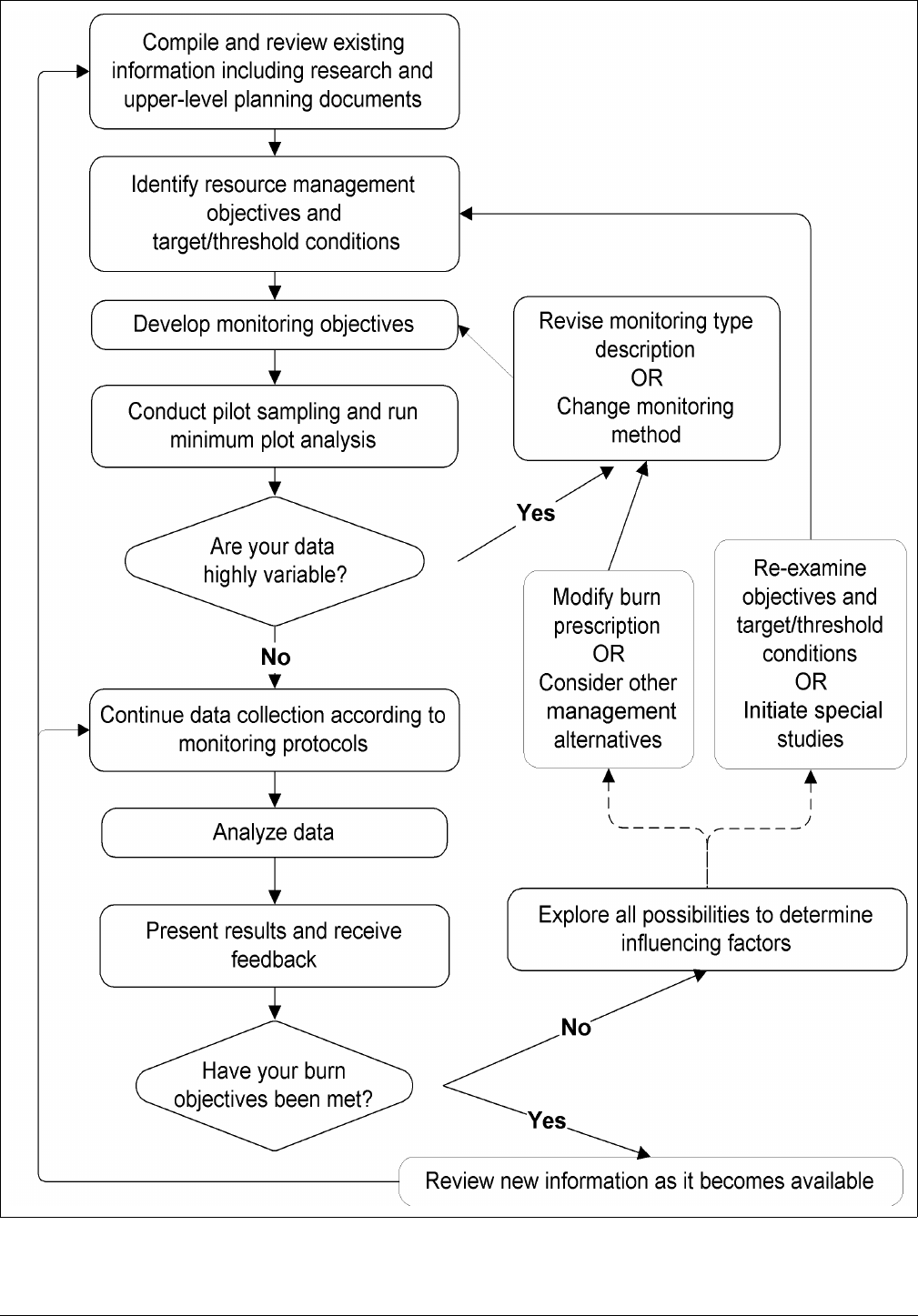
Figure 2. Steps in a fire effects monitoring program.

Fire Monitoring Handbook 18

3

Developing Objectives

“You got to be very careful if you don’t know where you’re going, because you might not get there.”

—Yogi Berra

Proper design is essential to any monitoring program.

The consequences of poor design are numerous, and

all bad. Lost time and money, unnoticed resource

deterioration, inadequate management decisions, and

reduced credibility are a few of the negative

repercussions of faulty planning and design. Take time

to design a program that will monitor the conditions

essential to meeting your management objectives.

Chapters three and four have been created to assist

you in the design of a high quality, defendable

monitoring program. By developing sound objectives

using the concepts put forth in Chapter 3, you will

build a solid foundation that will enable you to make

the necessary design decisions as covered in Chapter 4.

Natural area managers, like family physicians, should

monitor ecosystem health to prevent or identify

dysfunction and repair damage. Monitoring can tell

you the condition of the resource and detect change or

abnormal conditions. When you reintroduce a natural

process such as fire into the landscape, a monitoring

program will help you document any linkage between

the treatment and changes in resource condition, as

well as provide feedback on prescriptions and return

intervals.

The fire effects monitoring program flow diagram

(Figure 2, facing page) is designed to provide a concise

reference for the entire design, implementation and

analysis process involved in establishing an effective

fire effects monitoring program. It can be used as a

guide in the design of a monitoring program. Portions

of the flowchart will be expanded and detailed in this

and following chapters.

Development of a fire effects monitoring program,

including methodology and analytical techniques, must

be preceded by the development of fire-related

resource management objectives. The reduction of

hazard fuels, for example, should logically be

accompanied by fire behavior modeling using

postburn fuels data that demonstrate that the hazard

has in fact been abated, and that the stated fuel

reduction objectives have been met. This would

logically have been preceded by an analysis of the

nature of the hazard presented by the preburn fuel

characteristics.

Monitoring objectives are derived from resource

management and fire management program objectives.

From this, it should be apparent that fire managers and

resource managers must work together closely to

ensure that fire, whether managed as a natural process

or as a tool, is effective in meeting resource objectives.

Fire may meet fuel reduction objectives, for example,

but cause significant unwanted resource degradation.

19

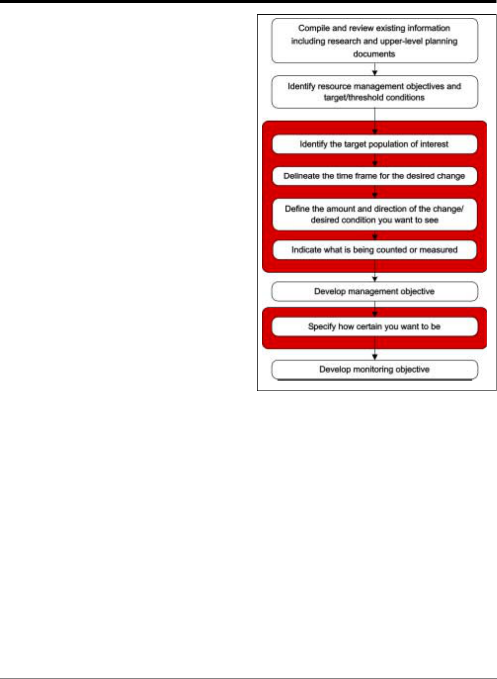
Objectives

MANAGEMENT OBJECTIVES

This handbook is organized around the development

of a monitoring program that is based on resource and

fire management objectives. Management objectives

are often misrepresented as goals (see the Glossary for

definitions of goal vs. objective). Developing clearly

articulated management objectives is a specific step

toward the accomplishment of a broader goal, and is a

critical step in any management-monitoring feedback

loop. This is true whether you use a more traditional

decision-making approach (such as those based solely

on cost, political considerations, or anecdotal

knowledge), or a more cooperative integrated

approach such as adaptive management (see below).

Management objectives serve as the foundation for all

activities that follow, including the proposed

management activity, monitoring, evaluation and

alternative management.

Objectives should be:

• Realistic and achievable. Create objectives that

are biologically meaningful and achievable within

the bounds of management possibilities. In addi-

tion, if you have multiple objectives, make sure

that they do not conflict. For example, you may

have trouble meeting both of the following objec-

tives: 1) dramatically reducing fuel load and 2)

maintaining all your overstory trees.

• Specific and measurable. Your objectives

should be quantifiable (measurable). They should

also identify a target/threshold condition or

include the amount and direction of change

desired. Specific quantitative elements will allow

you to evaluate the success or failure of your man-

agement.

• Clearly articulated and focused. Write clear

objectives that contain all the components

described on pages 22 (management) and 23

(monitoring), and presented in Figure 3. Clear and

focused objectives will allow current and future

stakeholders to have focused discussions regard-

ing the desired state of the resource.

Figure 3. Steps in developing management and monitoring

objectives

.

The key elements of an objective are highlighted in red.

Adaptive Management

Adaptive management is an iterative process—

planning, action, monitoring, evaluation, and

adjustment—which uses the results of management

actions as observations that help develop an enhanced

understanding of ecosystem response, in this case, the

effects of fire. Adaptive management is learning by

doing.

Adaptive management requires input from many

sources. By incorporating the views and knowledge of

all stakeholders—citizens, administrators, managers,

researchers—you create a working dialogue. In

establishing a working dialogue, you can articulate

sound management objectives, increase your ability to

implement management, gather reliable knowledge of

Fire Monitoring Handbook 20

all elements in the natural system of concern, and

make adjustments to management actions.

The adaptive process requires integrating the concepts

of observation, uncertainty, and surprise. Ideally, the

result will be not a single optimal state but a range of

outcomes, acceptable to all stakeholders, that avoid

irreversible negative effects on a highly valued resource

from the use of fire as a management tool.

Keep in mind that the process of setting objectives is a

dynamic process, and must include responses to new

information. It may be difficult to establish measurable

objectives due to lack of knowledge about a portion or

portions of the population, community or ecosystem

in question. Managers should use the best of available

information, and focus on creating knowledge-based,

measurable objectives.

Management Objectives and

Adaptive Management

As you learn more about the vegetative response to

fire, you will begin to have a better idea of the specifics

of the target/threshold conditions and how achievable

your objectives are. It is important to remember that

both management and monitoring objectives need

revisiting as a program evolves (see page 133).

As shown in the fire effects monitoring flow diagram

(Figure 2, page 18), as a general guide, objectives

should be reconsidered at least twice in a monitoring

cycle—this is the adaptive management approach (see

below, or review the references on page 238, Appendix

G.).

Planning Documents

The process of moving from broad, policy-related

goals to specific, quantifiable management objectives

can require steps at many levels. The steps taken to get

from tier to tier will vary from agency to agency, as

well as from park to park. Different methods will be

used to move through the “grey zone” from broad

goal to specific management objective. Prescribed fire

programs, and their objectives, are part of a larger,

multi-tiered framework of goals, target/threshold

conditions, strategies and objectives stated in the

General Management Plan (GMP), Resource

Management Plan (RMP), and Fire Management Plan

(FMP) for your unit.

The development of management objectives begins

with the policy and regulations that guide the agency.

Monitoring program managers may not refer to these

documents directly, but are familiar with their general

content. Guidelines and laws, such as the National

Environmental Policy Act (NEPA), the National

Historic Preservation Act (NHPA), and policy

guidelines established by a specific agency drive the

development of goals put forth in General

Management Plans and other management statements.

Again, these goals are expressed in broad terms.

A Resource Management Plan (RMP) and other

resource related documents (e.g., an ecological model

of the resource) will identify target/threshold

conditions, as well as problems that may prevent

managers from reaching the stated goals. What are the

problems that prevent managers from protecting and

perpetuating natural, scenic and cultural resources?

What impediments block managers from restoring

biological diversity? What is the target/threshold

condition or state of a forest stand or landscape unit?

A Fire Management Plan (FMP) outlines the strategy

of using fire to achieve the target/threshold

conditions. From the FMP, you will create specific fire

management objectives that will set measurable

criteria. The accompanying objective variables will

help you assess the effectiveness of treatment with

prescribed fire to meet those objectives.

Resource Management Plan

The need for prescribed fire, and what it should

accomplish, must be stated at least generally in the

RMP. This, in turn, should be supported by fire

ecology information which guides the development of

the FMP.

Perceived weaknesses in the value of monitoring data

may be due more to the lack of clarity of program

objectives than to flaws in the monitoring system.

Monitoring systems cannot be designed to monitor

everything, nor can they (without great cost) monitor

many things with a high degree of confidence.

Therefore, the value of monitoring is directly related to

a well-defined management objective.

Fire monitoring plan

The fire monitoring plan is where you record the

background information used to define your

management objectives, as well as additional planning

Chapter 3 n

nn

n Developing Objectives 21

information needed to drive your monitoring program.

The plan will include an ecological model that provides

a summary of what is known, as well as gaps in

knowledge, about the ecology of each species being

monitored (see page 225, Appendix F, for more

information on these models). The monitoring plan

should also include how management will respond if

you do not meet your objectives. Include in this

planning process any person who could influence a

change in management, both within the park and

external to the park. Create your plan with input from

fire and resources management specialists and field

technicians, and have it reviewed by your regional fire

effects program coordinator. The outline provided in

Appendix F should help you to develop an organized

plan for your park. RM-18 requires that all NPS

units applying prescribed fire must prepare a fire

monitoring plan (USDI NPS 2001a), regardless of

whether they use the protocols outlined in this

handbook.

Management Objective Components

Your planning documents should contain four key

components needed to create well-articulated

management objectives.

• Target population

•Time frame

• Amount and direction of change or target/threshold

condition

•Variable

Target population—monitoring type

Identify the target population, or portion of a

population, to be monitored.

• Carefully define the groups to be examined (e.g.,

species or group of species).

• Define the individuals to be included (e.g., should

you monitor every age class of all tree species in a

vegetation association or should you monitor only

the seedlings of a particular species?).

• Determine the geographic boundaries of interest

(for example, is the fuel load along the park

boundary the only fuel load of interest, or should

you collect data on fuels within one vegetation

association throughout the entire park?).

Identifying the target population provides a

quantitative picture of a plant association being

influenced by fire. It is the first step to creating a

monitoring type description (see Glossary). The

discussion on defining monitoring types begins on

page 34.

A five-year burn plan can be a starting point for

defining monitoring types. It will also play a role in

scheduling plot installation (see page 55). Burn units

identified in the five-year burn plan will help you

identify the target populations and the vegetation types

that are a high priority for monitoring type creation.

Time frame

Delineate the time frame for monitoring change. Use a

time frame that is realistic biologically (how rapidly will

the resource respond to fire?), as well as in terms of

management (how quickly can alternatives be

implemented in response to the trends indicated?).

The life history of the target organism will also help

you determine an appropriate time frame. In general,

long-lived, stable species will have longer monitoring

periods than short-lived, sensitive species. Also

consider the risk of rapid decline of a population,

either through loss of rare species or the establishment

of non-native competition.

Amount and direction of change or target/threshold

condition

Define the range of change (positive, negative, or no

change) you want to see or are willing to accept, or

state the actual target/threshold condition defined by

your management objectives. Again, the life history of

your target species and biology will dictate how much

change is possible and necessary. Because our

knowledge of fire ecology is poor for many plants and

plant associations, this is often the most difficult step

in this process. However, once you have determined

the direction of desirable change, determine a range of

acceptable target levels.

Examples:

Examples may include:

• Reduce mean (average) total non-native species

cover by 50–75%

• Maintain mean overstory tree density to within

10% of preburn

• Reduce mean total fuel load to less than 20 tons

per acre

• Increase the mean density of desired tree seed-

lings to 500 per hectare

Fire Monitoring Handbook 22

Variable

Indicate what you will count or measure in your

monitoring program. Describe the specific attribute

that the prescribed treatment will change or maintain.

When choosing a variable, consider the morphology

and life history of the species. Counting extremely

small, numerous individuals of a species may prove

costly, and because it is virtually impossible to do

accurately, variation in results may be an artifact of

sampling rather than a meaningful observation.

Examples:

Examples of variables may include:

• Fuel load—this can be broken down into size

classes or considered in total

• Percent scorch or percent mortality

• Density, frequency, relative or percent cover of a

given species or group of species

• Height of a given tree species, group of species

(by height class) or total understory

(See page 41 for additional variables)

Types of Management Objectives

Management objectives fall into two broad types,

change and condition. Each type of objective will

require different considerations for monitoring

objectives (page 23) and data analysis (page 130).

Change objectives

Use this type of objective when you want to track

relative change in a variable over time. This type of

objective is used when the trend over time is more

important than the specific current or future state, e.g.,

a reduction of 40% may be more important than a

decline to 500 individuals per hectare.

Examples:

The critical elements are highlighted:

• In the pine-oak forest monitoring type, we want

to reduce the mean total fuel load by 50–80%

within one year of the initial prescribed fire.

• We want to increase the mean percent cover of

native perennial grasses by at least 40%, in

tallgrass prairie, 10 years after the initial applica-

tion of prescribed fire.

Condition objectives

Use this type of objective when you have enough

information to describe a specific target/threshold

condition. Here you will measure your success by

considering whether your variable reaches a target or

threshold.

Examples:

The critical elements are highlighted:

• Within the cypress savanna monitoring type, we

want to decrease the mean density of

Taxo-

dium distichum

to less than 200 individuals per

hectare within six months postburn.

• In the ponderosa pine forest monitoring type,

we want to maintain a mean density of 90–120

overstory trees per hectare within five years of

the initial prescribed fire.

MONITORING OBJECTIVES

Monitoring objectives differ from management

objectives in that management objectives describe the

target/threshold or change in the condition desired,

while monitoring objectives describe how to monitor

progress toward that condition or change. Monitoring

objectives contain explicit statements about the

certainty of your results.

Development of sound monitoring objectives is a

critical step in any monitoring program. A common

mistake is for managers to collect data first and rely on

statistics to generate a question or objective later.

Certainty

Managers almost always need to rely upon incomplete

information to make decisions. Statistics can help

managers make decisions based on available

information. A carefully planned monitoring design

can ensure that you gather the data required for using

statistics appropriately to guide decision-making. Your

monitoring objectives will specify how certain you

want to be in your results.

For any monitoring program, a high degree of

certainty is desirable. Keep in mind, however, that

increased certainty often means increased money and

time. Fiscal and time limitations may restrict the

amount of sampling (number of plots), so you will

need to balance desired certainty with feasibility.

Sampling Principles

A true population value exists for every monitoring

variable. Measuring the entire population would reveal

the true value, but would likely be cost-prohibitive.

Chapter 3 n

nn

n Developing Objectives 23

Sampling procedures provide a method for reasonably

estimating these true values by measuring an adequate

portion of the population. The scientific method

provides a sound way to obtain a sample sufficient to

allow inferences to be made to larger populations. In

other words, when proper sampling procedures are

followed, data from monitoring plots (sample) are

used to infer results for the monitoring type as a whole

(population).

In most cases the entire population of interest cannot

be measured to determine the true population mean.

Since it is possible to determine the certainty with

which the sample estimates the true population value,

the protocols in this handbook involve sampling a

portion of the population. The greater the variability in

the sample data, the more uncertainty exists in the

estimation of true population values and differences

among populations. Generally, the larger the sample

size (number of plots), the greater the certainty.

Sample

The aggregate of all monitoring plots for a

particular monitoring type constitutes a sample.

An example of the layout of a sample is shown in

Figure 4. All monitoring plots within a given sample

are analyzed as a single data set. Monitoring plots are

randomly distributed throughout each significant

monitoring type occurring within the burn units that

are scheduled for burning within the next five years.

Due to fiscal and physical constraints, you cannot

install the number of plots needed for a high degree of

certainty (in the results) for every fire, or for every RS

variable. The use of a sample is specifically designed to

eliminate the need for plots in every prescribed burn

unit; this body of data should represent a large number

of burns and thus lessen the total amount of data

collected.

The sample database should not be used for

quantitative assessments of immediate postburn

effects or long-term change until all monitoring plots

comprising the sample have been treated. However,

analysis of those plots treated first can help you to

fine-tune your protocols, as well as to examine how

well you defined your monitoring type. Realistically,

depending on your burn schedule, it could take more

than five years to complete the immediate postburn

effects databases for a sample.

Figure 4. Graphical representation of a sample (all seven

monitoring plots combined).

Scientific method

Using the scientific method, sampling must follow

three principles: objectivity, replication, and

representativeness.

Objectivity—To be objective, or unbiased, sampling

must be random with respect to the question or

issue.

Example:

Plots are located randomly within monitoring types

(areas of relatively homogenous vegetation and fuel).

They are not, however, located randomly in all possi-

ble areas within a monitoring type, because only the

areas planned for prescribed burning are addressed

by the monitoring objectives. Locating plots in areas

that you do not plan on burning would be impractical

and would fail to serve the purpose of the monitor-

ing program. Finally, your monitoring type descrip-

tions should be written to limit the amount of

subjectivity in locating plots.

Replication—A replicated study includes sampling of

multiple units; measurement and treatment methods

are the same among sampling units.

Example:

Information from one monitoring plot, or from

multiple plots in one prescribed burn unit, will not

provide sufficient information about the effects of

prescribed fire. Additionally, measuring brush density

in a 1 m belt transect in one plot and a different belt

width in another would introduce variability in sam-

pling that could seriously confound the results. Simi-

larly, burning one plot, mowing another, and then

combining the data from the two, would not yield

clear results for either treatment.

Fire Monitoring Handbook 24

Representativeness—To be representative, the

observations or individuals measured must reflect the

population of interest.

Example:

Locating plots in areas that do not fit the monitoring

type would mean that the sample would not reveal

anything about fire effects in that monitoring type.

If these sampling principles are followed, then the

results from the sample can be used in inferential

statistics. This type of statistics attempts to provide

information about populations from information

gathered from a relatively small sample that has a

certain degree of variability.

Variability

In order to make inferences from the sample to the

larger population you must collect a sample that will

sufficiently estimate the population parameter of

interest as well as be objective, representative and

replicated. Knowing the variability of the data reveals

something about how good the sample (or estimate of

the population mean) is. If the data are not highly

variable (i.e., values for an objective variable, or

differences in these values over time, are very similar

from plot to plot), then it is likely that the sample mean

is a good estimate of the population mean. Highly

variable data (i.e., values for an objective variable, or

differences in these values over time, are very different

from plot to plot) means that it is less certain that our

sample mean is a good representation of the

population mean.

In either case, once you know the variability of your

data, you can calculate how many plots you need to

establish to provide a good estimate of the population

mean. If the natural variability of an objective variable

is high, then you will usually need more plots to

describe that variability. If the variability is low, then

you will find that fewer plots are sufficient to obtain a

reasonable estimate of the population mean.

Determining the minimum sample size based on

estimates of the population variability is discussed on

page 49.

Certainty Decisions

In designing a monitoring program, you will need to

make several choices related to certainty for each

objective variable, depending on the type of

management objective (condition or change (see page

23)). Make these choices carefully, because they will be

used to determine how many plots you will need to

achieve the desired certainty.

Change objectives

For change objectives, you want to determine whether

a change in the population of interest has taken place

between two time periods (for example, between

preburn and year-1 postburn). For change-related

management objectives, the monitoring objective will

specify:

• The minimum detectable change desired

• A chosen level of power

• A chosen significance level (alpha)

You will use these later to calculate the minimum

sample size needed to detect the desired change.

Minimum detectable change—The size or amount

of change that you want to be able to detect between

two time periods is called the minimum detectable

change (MDC). You need to determine how much of a

change is biologically meaningful for the population of

interest. Is a 10% change meaningful? 30%? 50%?

80%? Your management objectives should provide the

specific quantifiable levels of change desired. Looking

at these objectives, use the low end of a range of values

for your MDC. For example, if your management

objective states that you want to see a 50–80% change,

use 50% as the MDC.

The initial level of minimum detectable change, set

during the design phase, can be modified once

monitoring or new research provides information

about the size and rate of fluctuations of the

population. For example, you may discover that the

10% decrease in the mean percent cover of the

“nonnative” species you choose was not biologically

significant. This information might have come from

recent research that found the percent cover of this

species can fluctuate by more than 30% a year based

on weather conditions alone.

Minimum Detectable Change

If you choose a minimum detectable change amount of

less than 30%, consider reevaluating this decision.

Extremely variable populations may require a larger

sample than you can afford in order to detect these low

levels of change.

Chapter 3 n

nn

n Developing Objectives 25

Power—The amount of certainty that you want to

have in detecting a particular change is called power

(see page 127). You must determine how certain you

want to be of observing the desired minimum

detectable change.

Significance level—The probability that an apparent

difference occurred simply due to random variability is

called the level of significance, or α (alpha). You need

to decide the acceptable probability that the observed

difference was obtained by chance and is therefore not

attributable to the treatment.

Example:

These monitoring objectives are based on the exam-

ples of change management objectives on page 23;

the critical elements are highlighted:

• In the pine-oak forest monitoring type, we want

to be 80% certain of detecting a 50% reduction

in the mean total fuel load within 10 years of the

initial prescribed fire. We are also willing to accept

a 20% chance of saying that a 50% reduction

took place when it did not.

Here: power = 80%, MDC = -50%, and α = 20%

(0.20).

• In the tallgrass prairie monitoring type, we want to

be 95% certain of detecting a 40% increase in

the mean percent cover of native perennial grasses

within ten years of the first burn. We are willing to

accept a 5% chance of saying that a 40% increase

took place when it did not.

Here: power = 95%, MDC = +40%, and α = 5%

(0.05).

Condition objectives

If you want to determine whether the population of

interest achieves a stated condition, either a target or a

threshold, then you will use confidence intervals to

determine whether your objectives have been met. For

condition objectives the monitoring objective will

specify:

• The confidence level (i.e., the likelihood that the

confidence interval contains the true population

value, e.g., 80% or 95%)

• The desired precision level (closeness with which

the true population value is estimated)

You will use these later to calculate the minimum

sample size needed to ensure a certain probability that

your preburn and postburn sample means are within a

given percentage of the true preburn and postburn

means.

Example:

These monitoring objectives are based on the exam-

ples of condition management objectives on page 23;

critical elements are highlighted:

• Within the cypress savanna monitoring type, we

want to be 90% confident that the sample mean,

within six months postburn, of Taxodium distichum

density is within 25% of a true mean of less than

200 individuals per hectare.

• Within the ponderosa pine monitoring type, we

want to be 80% confident that the sample mean,

preburn and five years postburn, of overstory tree

density is within 25% of a true mean of 90–120

trees per hectare.

Confidence intervals—Certainty can be expressed

statistically by confidence intervals. A confidence

interval is a range of values that has a stated probability

of including the true population value for a variable.

This range of values, or confidence interval, is like a

measurement target with a certain probability that the

estimated true population mean falls somewhere on

the target.

Example:

A 95% confidence interval is a range of variable val-

ues which has a 95% probability of including the true

population value, i.e., approximately 19 out of 20

times (see Figure 5). An 80% confidence interval

means that there is an 80% probability that our con-

fidence interval includes the true mean value, i.e.,

approximately 16 out of 20 times (see Figure 6).

The mean value for a variable obtained from a sample

(all plots in a monitoring type) will always be located in

the center of this interval. The lower and upper ends

of the confidence interval are sometimes referred to as

confidence limits.

In the design of a monitoring program, you will need

to make two choices related to certainty for each

objective variable: the confidence level, and the desired

precision associated with the confidence interval.

These choices must be made carefully, because they

Fire Monitoring Handbook 26

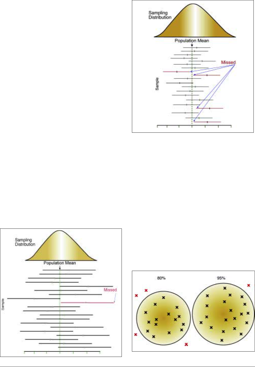
will be used to determine how many plots are needed

to achieve the desired certainty.

Confidence level—The confidence level is the

selected probability for the confidence interval (95%,

90%, or 80%). This level indicates the probability that

the confidence interval will include the estimated true

population mean (in other words, the probability of

“hitting the measurement target”). A critical

management decision involving ecologically or

politically sensitive species requires a high level of

confidence. For less sensitive decisions, managers

often may be willing to accept less certainty. General

guidelines for choosing the confidence level are as

follows:

• Choose an 80% confidence level for most objec-

tive variables.

• Choose a 90% or 95% confidence level if the

objective variable is potentially sensitive, or when

being confident of the monitoring results is criti-

cal (e.g., when a vital management issue is

involved, such as that regarding an endangered

species).

For a given sample size, the confidence level and

confidence interval width are directly proportional.

This means that if the confidence level increases

(increased probability of hitting the measurement

target), then the confidence interval is wider. Likewise,

if the confidence interval width is more narrow, it is

less likely that the target will be hit (lower level of

confidence) (see Figure 7).

Figure 5. 95% confidence intervals.

Figure 6. 80% confidence intervals.

There are two ways to increase confidence level

and reduce confidence interval width: increase the

sample size or decrease the standard deviation

(see Sampling Design Alternatives, page 48). Choosing

a confidence level and desired precision of the mean

will be used to calculate the number of plots needed to

achieve the desired certainty of the results.

Desired precision level—In addition to the

confidence level, managers must decide on the

precision of the estimate. The precision of a sample

statistic is the closeness with which it estimates the

true population value (Zar 1996). Do not confuse it

with the precision of a measurement, which is the

closeness of repeated measurements to each other.

The desired precision level is expressed as the width of

the maximum acceptable confidence interval. In the

Figure 7. Comparing 80% and 95% confidence interval

widths.

Chapter 3 n

nn

n Developing Objectives 27

case of most objective variables, the desired precision

level indicates how close the sample value is likely to

be to the true population value.

In the FMH software (Sydoriak 2001), the desired level

of precision is chosen by selecting a percentage of the

estimated population mean (e.g., must be <

25%). This

means that you are willing to accept a certain range

around the estimated value (e.g., the true mean is

within 25% of the estimated mean).

The precision selected should be related to the

need to have very close estimates of the true

population mean. General guidelines for choosing

the desired precision are as follows:

• Choose 25% precision for most objective vari-

ables when the exact values are not critical; if small

changes are not of a concern, then being within

25% of the true mean is probably sufficient.

• Choose 5–20% precision if the estimated mean

must be within a small percentage of the true pop-

ulation mean (e.g., if a population’s survival

depends on only slight changes).

Example:

In a deciduous northeast woodland, the sample mean

for the density of understory shrubs in 10 plots is

480 individuals per hectare. Managers need to be

accurate in their density estimates, because density is

a critical element of habitat suitability for the golden-

winged warbler, a species of concern. To keep sam-

pling costs down, but still collect data with a high

precision level, managers chose a confidence interval

width of 20% of the estimated true mean. In this

case, the acceptable confidence interval width is

within 96 individuals per hectare (plus or minus) of

the estimated true population mean. If the golden-

winged warbler, or any other species of concern, did

not inhabit this woodland, managers could use a

wider confidence interval width.

Precision

For the purposes of this monitoring program, the

desired precision cannot be greater than 25% of the

estimated population mean.

Fire Monitoring Handbook 28

Objective Variables

The Recommended Standard (RS) variables for

monitoring short-term and long-term change (levels 3

and 4) in the three plot types are outlined in Chapter

4 (see page 41). While each of these variables should

be monitored, you do not need to measure each with a

high level of certainty. A minimum level of certainty is

required, however, for a variable derived from each

management objective—a variable called the objective

variable (see Glossary).

Example:

If your primary management concern is to increase

the dominance of a suppressed shrub species, you

might choose only the percent cover of that species

for a high level of certainty, even though it is not the

dominant species in the preburn environment. You

would then use only this variable to calculate your

sample size. So the relationship between your objec-

tives and your objective variable might look like this:

• Management objective: We want to see a 40%

increase in the mean percent cover of all hazel spe-

cies (Corylus spp.), in eastern white pine forest, 5

years after the application of prescribed fire.

• Monitoring objective: We want to be 80% sure

of detecting a 40% change in the mean percent

cover of all hazel species (Corylus spp.), 5 years

after the application of prescribed fire and we are

willing to accept a 20% chance of saying a change

took place when it really didn’t.

• Objective variable: mean percent cover of all

hazel species (Corylus spp.).

You should monitor all the objective variables

contained within your monitoring objectives. Your

park natural resource specialist or ecologist, or a local

person with that expertise, is responsible for

identifying and defining the monitoring type, and for

creating monitoring objectives from your management

objectives. If local staff do not have the expertise

needed to make these decisions, you should seek

outside assistance.

Objective Variables

Not Covered by this Handbook

Your park’s fire management plan may specify

objectives that call for variables not discussed in this

handbook; for example: Increase the population of

raptors in all grasslands to >500 individuals. If park

management chooses objective variables that are

not covered in this handbook, you will need to

develop appropriate sampling methods. Appendix

G lists several monitoring references for other

sampling methods for organisms of special

management concern (e.g., forest insects and

pathogens, birds, reptiles, and mammals). These

references are limited, but should serve as a useful

guide. Take care to develop such customized

monitoring or research systems with the assistance of

subject-matter experts.

In addition, when choosing objective variables not

covered in this handbook, keep in mind that some

protocols may lend themselves to being sampled in

association with fire effects monitoring plots, e.g.,

songbird point counts. Integrating objective variables

as much as possible can be efficient and cost-effective.

Examples of Objective Variables

The objective variable that you choose should be the

most efficient measure of the change that you are

trying to achieve. The following are some potential

objective variables, some of which are recommended

(RS) variables (see Table 3, page 42).

Grasslands-brush—Percent cover for each of the

three most dominant species; percent non-native

species; density of shrub species.

Forest-woodland—Density of three most dominant

overstory trees; density of two dominant understory

trees; total fuel load; or any of those mentioned under

grasslands-brush.

Biological diversity—Species richness; diversity

indices.

Animal population dynamics—Birth-death rates;

number of individuals; size and shape of territory.

Chapter 3 n

nn

n Developing Objectives 29

Rare species occurrence—Number of individuals;

reproductive rates; dispersion. These types of variables

will be important if you are trying to enhance the

habitat of a rare species by burning.

Plant mortality and recruitment—Death and

establishment rates of selected plant species. These

variables could be very important in attempts to

encourage or discourage particular species.

The objective variables you chose to measure will

determine the sample size, and therefore labor costs,

for your monitoring program. Where there is a great

deal of variability among plots, a sparsely distributed

species, or a need for a high level of precision or

confidence in the results, the total number of plots

might be very high (see page 49 for a discussion of

minimum sample size).

COMPARING VEGETATION ATTRIBUTES

The following discussion will help you decide whether

to use density, cover or frequency for your objective

variable. This section also includes a discussion of the

point intercept method for measuring cover. Change

in all three of these variables may be expressed in

absolute or relative terms, e.g., percent cover and

relative cover. Use absolute values when you are

looking at how a variable changes on a per unit area or

sample basis. Use relative values when you are looking

at changes as a proportion of the total.

Density

Density is the number of individuals per unit area.

Density, used to estimate the abundance of a particular

species, is one of the most useful vegetational

attributes. Density is independent of cover, the

proportion of area covered by vegetation. For

example, two shrub species could have the same

percent cover where one consists of many small

individuals (high density) and the other of few large

individuals (low density). The adequacy of the sample

size for density measurements is dependent on the

shape and size of the plot used. Rectangular plots are

best to minimize the variation within plots for plants

with a clumped distribution. Since most plants grow in

clumps, rectangular plots may be your best bet. To

minimize the edge effect of non-circular plots,

establish an edge rule, e.g., 50% of the rooted base

must lie within the plot, or count plants with rooted

bases on one edge of the plot, but not those on the

opposing edge.

Advantages of using density as an objective

variable

• Density can be used to determine if the number of

individuals of a particular species is increasing or

decreasing.

• Density is an easily understood vegetational

attribute.

• If individuals are distinguishable, density measure-

ments are repeatable over time.

• Density is useful for monitoring threatened, endan-

gered, or sensitive plant species, because it samples

the number of individuals per unit area.

• Density is useful when comparing similar life forms,

e.g., two species of shrubs that are approximately the

same size.

Limitations of density measurements

• In some species, it can be hard to identify an individ-

ual. This is especially true for species that are capable

of vegetative reproduction, e.g., rhizomatous plants.

For such plants, measure stem density instead of the

number of individuals. No matter which is chosen,

the individual unit of interest must be objectively

identified and must remain the same throughout the

duration of the monitoring effort.

• Because plant species vary in size, density measures

lose a large amount of information about the plant

community being studied. For example, two species

may have identical densities, but the species that is

larger in size will appear to have the greater ecologi-

cal importance.

• Comparisons between densities of different growth

forms are meaningless; for example, densities of

trees and forbs cannot be compared.

• Seedling density, especially for herbaceous species, is

directly related to environmental conditions, which

can lead to misinterpretations of both positive and

negative trends.

Cover

Cover is an important vegetational attribute to which

ecologists have applied a wide range of meanings. One

of the most commonly used types of cover is canopy

cover, which is expressed as a percentage of the total

area measured, and defined as the vertical projection

of vegetation onto the ground surface, when viewed

from above. It is used in various ways to determine the

contribution each species makes to a particular plant

community. Cover measurement can provide a

quantitative and rapid measure for species that cannot

be effectively measured by density or biomass.

Fire Monitoring Handbook 30

Note: Typically, canopy cover of trees is assumed to

correlate with basal area or DBH. Relative dominance

also is used as a synonym for relative basal area or

relative cover.

Advantages of using cover as an objective variable

• Cover is one of the most widely used measures of

plant abundance because it is not biased by the size

or the distribution of the individuals.

• Cover provides a good indication of the relative

influence of a species.

• Cover measurements can be used for species in

which identification of individuals is difficult.

Limitations of cover measurements

• Cover, in herbaceous plants in particular, is very sen-

sitive to changes in climatic and biotic factors.

• Cover measurements favor species with larger leaves

or spreading growth forms. Additionally, species that

hold their leaves horizontally will have higher cover

values than species with acute or obtuse leaf angles.

• Because cover does not measure individuals, it does

not readily indicate changes in recruitment or mor-

tality.

Frequency

Frequency is a measure of the abundance and

distribution of a species. Frequency is the percentage

of all sampling units for which the canopy of a species

is present. Frequency is best measured by nested plots,

because it is very sensitive to plant size, dispersal

patterns and density. The point intercept method does

not measure frequency in the true sense of the word,

nor is it the best method to measure this variable.

Frequency is useful for monitoring changes in

vegetation over time, and for making comparisons

among different plant communities. Since it is a

variable that is not easily visualized across the

landscape, you should use it in addition to–but not in

place of–biomass, cover, or density.

Advantages of using frequency as an objective

variable

• Frequency sampling is highly repeatable, because it is

easier to determine presence or absence within a plot

than to measure cover or density.

• Frequency is a quick and inexpensive way to gather

statistical evidence of change in vegetation.

• Frequency is very sensitive to invasions of undesir-

able species.

• Frequency is also very sensitive to relative change

over time for key species.

Limitations of frequency measurements

• Frequency is influenced by the size and shape of the

quadrat used. What is an appropriate size for one

species will not be for another; thus nested quadrats

should be used in most frequency sampling. With

inappropriate plot shape and size, frequency can eas-

ily be over- or underestimated.

• To accurately determine change, the frequency for

the species in question must be between 20% and

80% (some say 30–70%).

• Frequency is very sensitive to changes that occur due

to seedling establishment. This can be offset by col-

lecting seedling information separately.

• Frequency is sensitive to changes in plant distribu-

tion in the sampled area, which hinders interpreta-

tion of changes.

• Interpretation of change is difficult because of the

inability of the observer to determine what attribute

of the vegetation changed. Frequency cannot tell you

if the change was due to change in basal area, plant

size, density, or pattern of distribution.

POINT INTERCEPT METHOD

The point intercept method uses the contact of a point

to measure cover. Many variations on this method

have been used to obtain estimates that are both

statistically sound and economically efficient. The

method used in this handbook is one such variation.

The theory behind this method is that if an infinite

number of points are placed in a two-dimensional area,

the exact cover of a plant species can be determined by

counting the number of points that hit that species.

This method then estimates the values from the

infinite number of points through the use of a sample

number of points.

Advantages of Using the Point Intercept Method

• This is considered the most objective way to mea-

sure cover—either a plant contacts the point or it

does not.

• Point intercept sampling is highly repeatable.

• This method is more precise than cover estimates

using quadrats.

• Point intercept sampling is more efficient than line

intercept techniques, especially for herbaceous vege-

tation.

• This is the best method for determining the cover of

the more dominant species.

• A minimum of training is needed to show field tech-

nicians how to lay out and read point intercept

transects.

Chapter 3 n

nn

n Developing Objectives 31

Limitations of the Point Intercept Method

• Sampling errors can occur if the pin is not lowered

plumb to the ground.

• Rare species with low cover values are often under-

sampled.

• Wind increases the time required for sampling.

• A large sample size is often required to obtain rea-

sonable accuracy and precision, especially for species

with low cover values.

• The technique can be slow.

• Use of the point intercept method is difficult in tall

vegetation types, because the “point” needs to be

taller than the vegetation.

OTHER METHODS

For an excellent reference on other methods of

measuring cover, and guidelines for when they are

appropriate, see Elzinga and others (1998 and 2001).

Fire Monitoring Handbook 32

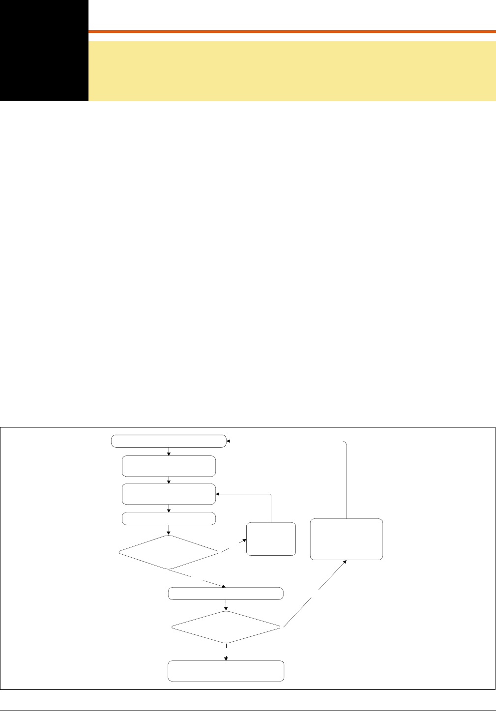
3

4

Monitoring Program Design

“To the person who only has a hammer in the toolkit, every problem looks like a nail.”

—Abraham Maslow

At the onset of the design of a monitoring program,

you will need to make a few basic decisions (see

Figure 8):

• Which attribute will best indicate whether each of

your management objectives (see page 20) was

met? Identifying this attribute, or objective vari-

able (see page 29), is a critical step in creating a

monitoring objective.

• What is the appropriate size and shape of each

sampling unit? See page 44 (Plot specifications)

for more details.

• How many plots do you need to monitor? See

page 49 (Calculating minimum sample size) for

more details.

You will make these decisions for each monitoring

type based on site-specific information and site-spe-

cific objectives. There is no such thing as one-size-fits-

all monitoring.

Once you have formulated a design, you can refine it

based on pilot sampling (see page 43). Pilot sampling

may reveal that it is impossible to address your objec-

tives within the time and money constraints of your

monitoring program. In such an instance, you could

refine your design in any of four ways:

• Change the type of monitoring to a less resource-

intensive type (which will have less statistical cer-

tainty), perhaps one that is more qualitative or

semi-quantitative (e.g., photo monitoring, cover or

density classes).

• Narrow the definition of the monitoring type (see

Glossary) and create two or more monitoring

types (e.g., split mixed grass prairie into Hesper-

ostipa comata–Carex filifolia and Bouteloua curtipen-

dula–Nassella viridula herbaceous vegetation

associations).

• Change the monitoring objectives (see page 23) to

less precisely estimate the variable on which your

minimum sample size is based, or modify them to

detect only larger changes.

• Modify your management objective so that you

can choose to measure a different vegetational

attribute.

Are your data

highly variable?

Develop monitoring objectives

Run minimum plot analysis

Revise monitoring type

description

OR

Change

monitoring method

Continue data collection as

per your monitoring protocols

No

Define monitoring types

& write descriptions

Establish plot protocols

and specifications

Conduct pilot sampling

Are plot sizes

and specifications

appropriate?

Revise

protocols

and

specifications

No

Yes

Figure 8. Steps in creating and refining monitoring type descriptions.

33

3

Monitoring Types

Using Chapter 3 as a general guide, you have worked

your way through the development of management

and monitoring objectives in the fire effects monitor-

ing flowchart (Figure 2, page 18). Once you have clear,

measurable objectives, your next step is to define the

population that you will monitor. For the purposes of

this handbook, this population is called a monitoring

type.

DEFINING MONITORING TYPES

A monitoring type is a major fuel-vegetation complex

or vegetation association that is treated with a particu-

lar burn prescription (which includes the season of the

burn), or a combination of a burn prescription and a

mechanical or other treatment, e.g., browsing, grazing,

herbicide, seeding, or thinning. For example, a moni-

toring type could be defined as: a red pine dominated

(>

50% of the mean total basal area) conifer forest, fuel

model 9, burned in the spring during green-up.

Defining a monitoring type requires considerable judg-

ment. It should be done after careful field reconnais-

sance and in consultation with a fire or vegetation

ecologist. The process as defined in this handbook

calls for stratifying monitoring types by selecting

appropriate defining and rejecting criteria.

Each monitoring type must be relatively homoge-

neous. If a monitoring type is not homogeneous, its

high level of variability will likely indicate the need for

a unreasonably high number of monitoring plots.

However, if a monitoring type includes vegetational

complexes of similar composition spread across a

changing landscape, then it might include a range of

stand densities, structure, fuel load, understory, and

herbaceous associates.

If a monitoring type includes vegetation complexes of

similar species composition, but the conditions that

relate to your management objectives (e.g., fuel load)

vary across the type, then there are two ways to reduce

statistical variability:

• You can create highly variable monitoring types

that may require a large number of plots within

each monitoring type to pick up the within-sample

variability. However, this may reduce the total

number of plots that are rejected in the field.

• You can create strictly homogeneous monitoring

types that can decrease the sample size within a

type, but could dramatically increase the total

number of plots needed to monitor the greater

number of monitoring types being used.

Example:

Two types of white pine forest are intermingled

throughout a park, one dominated primarily by white

pine, and another with a mixture of eastern hemlock

and hardwoods. The management objective for both

plant associations is to create a forest with a mean

density of overstory white pine between 75–110 indi-

viduals per hectare within 50 years of the initial treat-

ment. Park managers may want to consider lumping

these two plant associations together into one moni-

toring type. Lumping these two associations will

probably reduce monitoring costs by decreasing the

total number of plots and by increasing sampling

efficiency, as monitors will be less likely to reject

plots that contain the intermingled forest types.

Define the minimum number of monitoring types that

will represent the major fuel-vegetation complexes or

vegetation associations within the units that you will

manage using prescribed fire. Try to resist the tempta-

tion to identify all possible types. A park of moderate

topographic and vegetational complexity could easily

have 50 to 100 possible types using the criteria listed

above; however, this creates an impractical monitoring

design. The necessary compromise should be devel-

oped with the assistance of a vegetation management

specialist and/or fire ecologist. You will then further

refine each monitoring type through pilot sampling

(see page 43).

Fire Monitoring Handbook 34

Monitoring Types

In the interest of efficiency, start with highly variable

monitoring types, and then divide them if necessary.

Start by delineating a type where your objectives are

the same or similar. Then, look at the variability of

your objective variables within that type. If there is a

wide range of values for these objective variables, then

it may be wise to further divide your type. If not, keep

the type as is.

If you know of another park that has similar vegetation

types, management objectives, burn prescriptions, etc.,

consider using that monitoring type description,

including any changes necessary to compensate for

local differences. This can potentially reduce the total

number of plots needed in each park. If another park

has similar vegetation types, but different objectives,

you should at least review their monitoring type

descriptions to see where your similarities lie.

Step 1: Establish Selection Criteria

The first step is to establish the specific criteria used to

identify each monitoring type. By defining selection

criteria, monitors can determine whether each ran-

domly selected monitoring plot is truly representative

of the type. Defining criteria quantitatively (e.g., >75%

basal area of table mountain pine with <30% white

oak; or >60% cover of blackbrush with <10% cover

of Joshua tree) should permit a qualitative or even

quantitative comparison of trends among monitoring

types or even among similar monitoring types from

different parks.

Types may be differentiated on the basis of one or a

combination of the following elements:

Vegetation composition

Vegetation composition is defined, according to a fed-

eral standard (FGDC 1996), by the mixture of plant

species that form a community. Plant community is a

general term that can be applied to any vegetation unit,

from the regional to the very local. A qualified

resource manager or researcher establish the range and

limits of compositional variability for any named plant

community (e.g., association, alliance). Examples are

Quercus gambelii–Amelanchier alnifolia shrubland associa-

tion, Danthonia intermedia-Solidago multiradiata herba-

ceous vegetation association, and Quercus virginiana-

Sabal palmetto forest alliance. For the current list of fed-

eral standard plant associations, see The Nature Con-

servancy (1998) on the subject.

Vegetation structure

Vegetation structure refers to the distribution of the

composite elements—i.e., how abundant various plant

species are within a plant association, and how many

different layers they form. Examples of vegetation

structure are: dense herbaceous cover within a forest

type; pine with scattered shrubs; oak stands without

reproduction with a continuous non-native grassland

understory; dense cover of native perennial bunch-

grasses; and dense palmetto with scattered slash pine.

Sensitive species

Monitoring types are occasionally defined by individual

species that are considered sensitive due to environ-

mental, political or other factors. For example, some

biotic elements are adapted to a strict fire regime or are

extremely sensitive to a certain type of fire. Some areas

may require a fire regime very different from the norm

for that vegetation type in order to respond to political

concerns. Examples of sensitive elements are: endan-

gered plant populations or habitat, politically or envi-

ronmentally sensitive species or habitats, and popular

habitats such as giant sequoia groves or vernal pools.

Physiography

Topography is often critical for identifying the distri-

bution of small monitoring types, especially if the types

include rare species. Physiographic changes in slope,

aspect, topographic position, or elevation can define a

monitoring type. Stratification based solely on these

elements for larger monitoring types, however, is gen-

erally inappropriate, since the biological elements fre-

quently cross physiographic “boundaries,” or occur

over a broad range of conditions.

Fuel characteristics

If the strata in your park vary significantly, you may

divide classic (Anderson 1982) or custom fuel models

into different monitoring types. Examples are change

in dead and downed loads, standing fuel density, duff

loads, biomass, height, and continuity. Conversely, you

may include multiple vegetation types within a single

fuel model.

Burn prescription

Burn prescriptions identify desired fire behavior (e.g.,

flame length) and amount of fuel consumption and

smoke production, and therefore predict expected

burn results. Burn prescriptions also define the fre-

quency (the return interval) and the season of the

burn. Examples of how a burn prescription might dif-

Chapter 4 n

nn

n Monitoring Program Design 35

ferentiate a monitoring type are: a shrub association

being burned in the spring in one part of the park and

in the fall in another part of the park, or a perennial

grassland being burned with a frequent return interval

(1–4 years) in one area, and on a longer fire return

interval (7–15 years) in another. Note that in each of

these examples, you would need different management

objectives to truly separate these types.

Other treatments

Occasionally, managers use other tools in conjunction

with fire to achieve management objectives. These

might include browsing, grazing, herbicide, thinning,

or seeding. Areas subject to more than one type of

treatment should not be lumped with prescribed fire-

only treatments.

Plot type

When choosing a plot type (forest, brush or grassland),

keep in mind your objective variable or other variables

you want to measure. If you need to use forest plot

protocols (e.g., to track the height of tree-like shrub

individuals), use a forest plot even in a treeless moni-

toring type. Note: If you use a forest plot in this situa-

tion, use only the protocols that you need and

disregard the rest.

Additionally, think about the future structure, compo-

sition and characteristics of your monitoring type.

Using a forest plot in a grassland area is appropriate if

you intend to monitor the encroachment of trees into

an area. Likewise, you would use a brush plot to moni-

tor the encroachment of shrubs into a grassland area.

You can use grassland plots to monitor the encroach-

ment of non-native species into native grassland, or to

capture the migration of a species into or out of an

area.

Step 2: Describe the Monitoring Type

A detailed description of each monitoring type is

essential to define the appropriate location for moni-

toring plots, monitor the biophysical elements of con-

cern, and qualitatively and/or quantitatively compare

variables between areas or plots.

On the Monitoring type description sheet (FMH-4 in

Appendix A) record all of the following information

(see page 39 for an example):

Park unit 4-character alpha code

This is the four letter code given to every National

Park unit, generally designating the first two letters of

the first two words, or the first four letters if only one

word, e.g., NOCA = North Cascades National Park, or

BAND = Bandelier National Monument.

Monitoring type code

Each monitoring type must be identified by a stan-

dardized code to facilitate computerization and com-

parative analyses within and among NPS units.

Assign a unique multi-character code as

described here:

Plot Type: F = forest, B = brush, G = grassland

Dominant Species Code (see page 83): if no clear dom-

inant exists, or if you have more than one monitoring

type with the same dominant, create your own code,

e.g., MIPR1 = mixed prairie.

Burn Season Phenology (phenological stage of key

plants affected by or carrying the fire during a burn (a

burn prescription element)):

G = green-up (period of active plant growth)

T = transition (active growth phase nearly over; plants

setting and dispersing seed)

D = dormant (plants cured, dormant; deciduous trees

lost leaves)

Fuel Model: #01–13 or custom model

Examples:

FSEGI2T08—(forest plot, dominated by Sequoiaden-

dron giganteum, burned during transition, fuel model 8)

BCLMAJG03—(brush plot, dominated by Cladium

mariscus ssp. jamaicense, burned during green-up, fuel

model 3. Note that here managers are using a brush

plot in a “grassland” plant association to track the

encroachment of shrubs)

GAGCRD01—(grassland transect, dominated by

Agropyron cristatum, burned when dormant, fuel

model 1)

Monitoring type name

Use a name that most people will recognize as repre-

senting the plant association(s) in which you are work-

ing. For example, chamise chaparral, Madrean pine-oak

woodland, northern pine barrens.

FGDC (Federal Geographic Data Committee)

association(s)

Note the federal standard plant association(s) (FGDC

1996; The Nature Conservancy 1998) that your moni-

Fire Monitoring Handbook 36

toring type description encompasses. For example,

Andropogon gerardii–Panicum virgatum Dakota sandstone

herbaceous vegetation, Artemisia tridentata–Chrysotham-

nus nauseosus shrubland. Consult state, agency, The

Nature Conservancy or other ecologists involved in

developing local level association descriptions if you

have any doubt as to the names of plant associations in

your area.

Burn prescription

Provide detailed information regarding the prescrip-

tion and any other management treatments (as dis-

cussed on page 35) that you will use throughout the

type. Note: Include the full range of conditions under

which you will burn the type.

Objectives

Management objective(s)—Include your manage-

ment objective(s) as discussed on page 20.

Monitoring objective(s)—Include your fire monitor-

ing objective(s) as discussed on page 23.

Objective variable(s)

It is strongly suggested that you monitor one variable

to a chosen level of certainty for every management

objective. For a more complete discussion of objective

variables, see page 29.

Physical description

Describe the physical elements selected in Step One

(page 35) that characterize the type. This includes the

range of geologic and topographic features included in

the type—soil type(s), aspect(s), elevational range, gra-

dient, landforms, etc.

Biological description

Quantitatively and qualitatively describe the species

that dominate or characterize the vegetation associa-

tion selected in Step One (page 35). Indicate the

acceptable range of values for the elements that define

each stratum.

Rejection criteria

Establish rejection criteria that would make a potential

plot site unsuitable for monitoring. Note that your

rejection criteria may differ among monitoring types;

rejection criteria for one monitoring type may in fact

be representative of another type. Examples of possi-

ble rejection criteria include:

• High percentages of rock outcrops, barren spots,

soil, and/or vegetation anomalies (e.g., a small

meadow in a forest)

• Locations close (<30 m) to a road, trail, potential

development site, proposed fireline, developed

area, or monitoring type boundary (ecotone)

• Areas to be blacklined or manually cleared before

burning (unless the entire burn unit is to receive

this “treatment”)

• Evidence of more recent fire than that in rest of

the monitoring type

• Inclusion of archeological sites

• Areas with >50% slope (installing and monitoring

plots on steep slopes can result in excessive dam-

age to the herbaceous vegetation and fuel bed.

Where practical, it is recommended that you avoid

such slopes)

• Threatened or endangered species habitat that

park management wants to protect from fire

• Substantial disturbance by rodents, vehicular traf-

fic, or blow downs, volcanic activity, etc.

• Intersection by a stream; seep or spring present

• Safety issues, e.g., known high density rattlesnake

habitat

• Inventory, monitoring, or research plots that

would be compromised by the co-location of plots

• Other locally defined conditions that present

problems

By establishing clear monitoring type descriptions and

rejection criteria, you can avoid bias. Examples of rea-

sons not to reject monitoring plot locations:

• Not typical: Plot location is thought to be atypical

(a plot is either in the type or not; it should be

rejected only because it does not meet the monitor-

ing type description)

• Too difficult to sample: It would be too difficult to

put in transect at this location (shrubs too dense, or

plot location is hot and lacking shade trees)

Notes

In this section, identify any deviations from or addi-

tions to protocols listed in this handbook. Describe

your pilot sampling design as well as any special sam-

pling methods, including any variation in plot size or

shapes to accommodate individual species. This sec-

tion should also note any species for which you will

collect DRC instead of DBH, and list any shrub spe-

cies that are clonal or rhizomatous, and therefore not

counted in the belt transects.

Additional headers

If you recreate your Monitoring type description sheet

using a word processing software program you may

find it useful to add other sections, such as: “Vari-

able(s) of Interest” (any variable of concern you might

Chapter 4 n

nn

n Monitoring Program Design 37

want to track, but not necessarily to a chosen level of

certainty) or “Target Condition” (attributes that you

are using fire management to maintain or restore).

Plot protocols

On the second page of the Monitoring type descrip-

tion sheet (FMH-4 in Appendix A), indicate the

optional variables to be measured, the areas in which

Recommended Standard (RS) variables are to be mea-

sured, and all other protocols that apply to each indi-

vidual monitoring type. See the example in the next

column.

Example:

The plot protocols example on page 40 indicates that

you:

• Use abbreviated tags, collect voucher specimens,

and install all 17 stakes

• Measure the following optional variables preburn:

herbaceous height, tree damage (live only), over-

story crown position (live and dead), pole-size and

seedling tree height, and dead seedling density

• Sample the following areas:

• Q4–Q1 and Q3–Q2 for herbaceous cover

• species not intercepted but seen on both sides of

the herbaceous transect—5 m wide on both her-

baceous transects

• shrub density—5 m wide belt transect on both

herbaceous transects

• overstory trees—all quarters of a 50 × 20 m plot

• pole-size trees—Q1

• seedling trees—a 5 × 10 subset of Q1

• fuel load—6, 6, 12, and 50 foot transects

• Measure the following optional variables during

the burn: duff moisture and flame depth

• Collect burn severity data along the fuel transects,

and measure the following optional variable

immediately postburn: char height

Pilot Sampling and Monitoring Types

Monitoring type selection and description will be

tested, and may be modified, during a process known

as pilot sampling (see page 43). This process of fine-

tuning uses a range of plot protocols and a limited

number of plots to ascertain the extent of variability

within a monitoring type and among the variables of

importance that have been selected.

Example:

A monitoring type description should include the

level of effort and quantitative information found on

the next page.

Fire Monitoring Handbook 38

FMH-4 MONITORING TYPE DESCRIPTION SHEET

Park: DETO

Monitoring Type Code: F P I P O T 0 9

Date Described: 1/10/01

Monitoring Type Name: Ponderosa Pine Forest

FGDC Association(s): Pinus ponderosa – Quercus macrocarpa Woodland; Pinus ponderosa – Prunus

virginiana Forest

Preparer(s): G. San Miguel, B. Adams, G. Kemp, P. Reeberg

Burn Prescription (including other treatments): Units will be burned between Labor Day and the end

of September. Flame length 0.5–3 ft; rate of spread 0–3 ch/hr. Temperature 30EÐ85EF.; Relative humidity

25–55%; Midflame wind speed 0–20 mph; Fuel moisture as follows: 1-hr 6–14%, 10-hr 8–15%, 100-hr

10–30%.

Management Objectives: Reduce the mean total fuel load by 50–80% immediate postburn and main-

tain for at least two years postburn; reduce mean overstory density by 20–40% by the fifth year postburn;

and increase the mean herbaceous and shrub cover by 25–45% within 10 years postburn.

Monitoring Objectives: We want to be 80% confident of detecting a 50% decrease in the mean total

fuel load (immediate and two years postburn), and a 20% reduction in the mean density of all overstory

trees, five years after the application of prescribed fire. For both of these objectives we are willing to

accept a 20% chance of saying these reductions took place when they really did not. In addition, we

want to be 90% confident of detecting a 25% increase in the mean percent cover of understory species

and we are willing to accept a 10% chance of saying that this increase took place when it really did not.

Objective Variable(s): Mean total fuel load; mean density of overstory ponderosa pine; mean total

understory cover.

Physical Description: Includes upland sites on all aspects and slopes with an elevation from 4,000' to

6,000', which includes upper, mid and lower slopes. Talus slopes and steep slopes (>40% slope) are

excluded. Characteristic soils consist of deep, well-drained clay, or sandy loam of the Larkson–Lakoa

Series. There are also some areas of exposed sandstone.

Biological Description: Overstory dominated (greater than 65% of the canopy cover) by ponderosa

pine (Pinus ponderosa). Understory trees (15–60% cover) include: bur oak (Quercus macrocarpa),

chokecherry (Prunus virginiana), and American plum (Prunus americana). Shrubs (0–30% cover)

include: Oregon grape (Mahonia repens), common juniper (Juniperus communis), pink current (Ribes

cereum). Grasses and forbs (0–20% cover) include: poverty oat grass (Danthonia spicata), needle and

thread (Stipa comata), Western wheatgrass (Agropyron smithii), big bluestem (Andropogon gerardii),

and Kentucky bluegrass (Poa pratensis).

Rejection Criteria: Large outcroppings or barren areas >20% of the plot; areas with anomalous vegeta-

tion; monitoring type boundaries; riparian areas; areas dominated by deciduous trees (>30% cover);

areas within 30 m of roads, burn unit boundaries, or human made trails or clearings; and areas within 20

m of woodlands. Research exclosures are to be rejected.

Notes: Do not collect shrub density for Oregon grape because it is has underground stolons, and there-

fore it is difficult to identify individuals for this species.

Chapter 4 n

nn

n Monitoring Program Design 39

FMH-4 PLOT PROTOCOLS

GENERAL PROTOCOLS (Circle One) (Circle One)

Preburn

Control Treatment Plots (Opt)

N

Herb Height (Opt)

Y

Herbaceous Density (Opt)

N

Abbreviated Tags (Opt)

Y

OP/Origin Buried (Opt)

N

Herb. Fuel Load (Opt)

N

Voucher Specimens (Opt)

Y

Brush Fuel Load (Opt)

N

Count Dead Branches of Living Plants as Dead (Opt)

N

Width Sample Area for Species Not Intercepted But Seen in Vicinity of Herbaceous

Transect(s):

5 m

Length/Width Sample Area for

Stakes Installed:

All

Shrubs:

50 × 5 m

Herbaceous Frame Dimensions:

Not Applicable

Herbaceous Density Data Collected At:

Not Applicable

Burn

Duff Moisture (Opt)

Y

Flame Depth (Opt)

Y

Postburn

100 Pt. Burn Severity (Opt)

N

Herb. Fuel Load (Opt)

N

Herbaceous Data (Opt): FMH- 15/16/17/18:

Do Not Collect

FOREST PLOT PROTOCOLS (Circle One) (Circle One)

Overstory

Live Tree Damage (Opt)

Y

Live Crown Position (Opt)

Y

(>15 cm)

Dead Tree Damage (Opt)

N

Dead Crown Position (Opt)

Y

Record DBH Year-1 (Opt)

N

Length/Width of Sample Area:

50 × 20 m

Quarters Sampled:

Q1

w

Q2

w

Q3

w

Q4

Pole-size

Height (Opt)

Y

Poles Tagged (Opt)

N

(>2.5<15)

Record DBH Year-1 (Opt)

N

Dead Pole Height (Opt)

N

Length/Width of Sample Area:

25 × 10 m

Quarters Sampled:

Q1

Seedling

Height (Opt)

Y

Seedlings Mapped (Opt)

N

(<2.5 cm)

Dead Seedlings (Opt)

Y

Dead Seedling Height (Opt)

N

Length/Width of Sample Area:

10 × 5 m

Quarters Sampled:

Subset

Herbaceous

Cover Data Collected at:

Q4–Q1

w

Q3–Q2

Fuel Load

Sampling Plane Lengths:

6

1 hr w

6

10 hr w

12

100 hr w

50

1,000 hr-s w

50

1,000 hr-r

Postburn

Char Height (Opt)

Y

Poles in Assessment (Opt)

N

Collect Severity Along: Fuel Transects

Fire Monitoring Handbook 40

Variables

Variables (see Glossary) are monitored by sampling

according to a standardized design. Customized meth-

ods may also be needed for special concerns; however,

your regional ecologist and/or fire effects monitoring

specialist should review any customized methods or

form modifications.

LEVEL 3 AND 4 VARIABLES

Procedures for monitoring levels 3 and 4 are similar,

but differ in timing and emphasis. The Recom-

mended Standard (RS) for monitoring short-term

change (level 3) is to collect detailed descriptive infor-

mation on fuel load, vegetation structure, and vegeta-

tion composition. This information is determined only

broadly at level 2, Reconnaissance–Fire Conditions.

Wildland fire management may also require the collec-

tion of some or all of these data.

If your program has both short-term and long-term

management objectives, you may be required to use

different variables and different monitoring frequen-

cies for monitoring levels 3 and 4. For example, a man-

agement objective of using fire to open up a woodland

stand and improve native grass and forb populations

by reducing the density of live pole-size trees would

require a monitoring objective to assess the mortality

of pole-size trees preburn to immediate postburn. A

short-term (level 3) objective variable could be live

pole-size tree density. To assess the herbaceous

response preburn to year-2, or even year-5 postburn, a

long-term (level 4) objective variable could be herba-

ceous cover. The objective variable contained within

the long-term objective becomes the long-term RS for

level 4 monitoring.

If a program has only short-term management objec-

tives (for example, to reduce fuel load or shrub den-

sity), the RS for level 4 monitoring is to continue

monitoring all level 3 variables over an extended

period of time. Both situations include using the

change over time minimum sample size equation (see

pages 49 and 124 for discussion; for formula, see page

217 in Appendix D) for all objective variables using the

time periods specified in your management objectives.

A monitoring program can and should be customized

to address specific park needs; however, any modifica-

tions in the program must be approved by your park’s

resource management specialist and fire management

officer, and reviewed by a park scientist or local

research scientist. These proposed changes should

then be sent to your regional office for review.

Monitoring for long-term change requires collecting

information on trends, or change over time, in an eco-

system. Such change can be neutral, beneficial or detri-

mental. If your monitoring program detects a trend of

concern, you can implement a research program or

appropriate management response to obtain more

information. For example, the National Park Service

did not formally conduct long-term monitoring during

its policy of fire suppression up until 1968. As a result,

undesired effects in many parks were not formally rec-

ognized for about 90 years, and only after considerable

(and often irreversible) damage had been done. With a

systematic process of monitoring and evaluation, man-

agers might have reevaluated the suppression policy

earlier. Similarly, current fire management strategies

also have the potential to cause undesired change. For

this reason, long-term monitoring should accompany

all types of fire management strategies.

The existence of a long-term trend is revealed by con-

tinued monitoring of the short-term (level 3) objective

variables. Select objective variables that are good indi-

cators of both short-term and long-term change. This

handbook does not specify the most appropriate indi-

cators of long-term change, as they will be different

for each park and monitoring type. Park staff should

select objective variables (with input from resource

management specialists and other scientists as needed)

by examining 1) fire management goals and objectives,

2) their biota’s sensitivity to fire-induced change, and

3) special management concerns.

The RS variables listed should be monitored according

to the monitoring schedule (for the schedule of level 3

and 4 variables, see page 57). Monitoring methods and

procedures for monitoring plots are described in

Chapter 5.

RS VARIABLES

Recommended Standard (RS) variables (Table 3, next

page) can be used to track both short-and long-term

change in the vegetation and fuel components of your

ecosystem. After following these variables over the

Chapter 4 n

nn

n Monitoring Program Design 41

long term, while only a few will have a high level of

certainty, the results from all variables will help you

identify topics for follow-up research or necessary

changes in your monitoring objectives or sampling

protocols.

Example:

In a sugar pine (Pinus lambertiana) monitoring type,

the objective variables are the density of overstory

sugar pine and total fuel load. After collecting data

for five years, the fire manager notices that the mean

percent cover of Ribes nevadense is 30 times the preb-

urn cover. The manager suspects that the fire has

caused this increase and is concerned since Ribes

nevadense is an alternate host for the non-native white

pine blister rust, which kills sugar pines.

In this example, the manager recognized a trend based

on a variable (mean percent cover of Ribes nevadense)

that was not an objective variable. The manager now

must determine whether the measured increase in Ribes

nevadense is either biologically significant (does this

change in cover necessarily increase the threat that

these shrubs will spread blister rust?) or statistically

significant. The next step might be to install control

plots, examine plots from other studies (outside of the

burned area, but within the monitoring type), or ini-

tiate a research study to address this issue.

Table 3. Recommended Standard variables for monitoring

(level 3 & 4) grassland, brush, and forest plots.

Plot Type Variables

Grassland

• Percent cover by species

• Relative cover by species

• Number of non-native species

• Number of native species

• Burn severity

Brush or

Shrubland

All grassland variables, plus

• Shrub density by species

• Shrub age by species

Forest or

Woodland

All grassland and brush variables, plus

• Tree density by species

• Tree diameter by species

• Fuel load by size class

• Total fuel load

• Duff depth

• Litter depth

• Average scorch height

• Percent of crown scorched

Fire Monitoring Handbook 42

Sampling Design

PILOT SAMPLING

Once you have defined your monitoring type, you will

fine-tune it with a process called pilot sampling. This

initial step will help you determine whether your plot

sizes and/or shapes are appropriate, and whether the

protocols discussed in this handbook are appropriate

for your park.

The first step in pilot sampling is to collect and analyze

field data. While you are collecting and entering these

data, consider the questions listed under “Consider-

ations Prior to Further Plot Installation” (page 47). If

your answers to any of these questions is “no,” you

should explore sampling design alternatives.

Install ten initial plots in a monitoring type using the

restricted random sampling method discussed on page

59. Then analyze all plot variables and adjust your sam-

pling design as necessary. If the density of the species

being sampled (trees, shrubs or herbs) is relatively

high, use smaller sampling areas (eliminating the

counting of hundreds of plants in each plot) through-

out the monitoring type. Conversely, if the density is

relatively low, use a larger sampling area to avoid hav-

ing a sampling area in which no plants occur. See pages

44–47 for some guidelines to follow when making

these decisions.

In addition, calculate the coefficient of variation (see

Appendix D, page 218, for the equation) for each vari-

able (not just your objective variable(s)), checking to

see which size-shape combination gives you the lowest

coefficient of variation. This will help you decide on

the most efficient design for your sampling areas.

Note: Also use this process if you are using different

sampling attributes or areas postburn. After adjusting

sampling areas and revisiting plots to resample, you

can calculate minimum sample size (see page 49).

Sampling Area Consistency

Once you have refined the size and shape of a sam-

pling area for a variable through pilot sampling, do not

change the sampling area. Sampling area (size and

shape) must be consistent among plots within a moni-

toring type, and should be consistent for each variable.

If the size or shape of the sampling area is changed, all

plots installed prior to the change must be revisited so

that every plot within a monitoring type has the same

sampling design.

Redesigning an Existing

Sampling Design

If you have plots that were established without using

the pilot sampling process, you might be able to reas-

sess your sampling design, provided that you have

well-documented data sets. For example, if you have

excellent pole-size tree maps, then you can conduct

pilot sampling by trying different plot shapes and sizes

on your maps. If you have poor maps, or you find that

you need larger sampling areas, consult with a special-

ist in sampling design before you make any changes to

your study design.

Pilot Sampling

When you visit the first plots in a monitoring type,

sample pole-size and seedling trees as well as shrubs in

a larger area, and map the location of each tree or

shrub (or separate the brush belt into smaller widths).

This way when the ultimate sampling area is chosen

you can refer to the map (or smaller belt width) and

delete the data that do not belong in this final sampling

area without having to revisit the plot. This is a good

tip for situations where you end up using a “larger”

area or an “unusual” plot shape, or the plot is difficult

to access. It may be inefficient in other cases.

Chapter 4 n

nn

n Monitoring Program Design 43

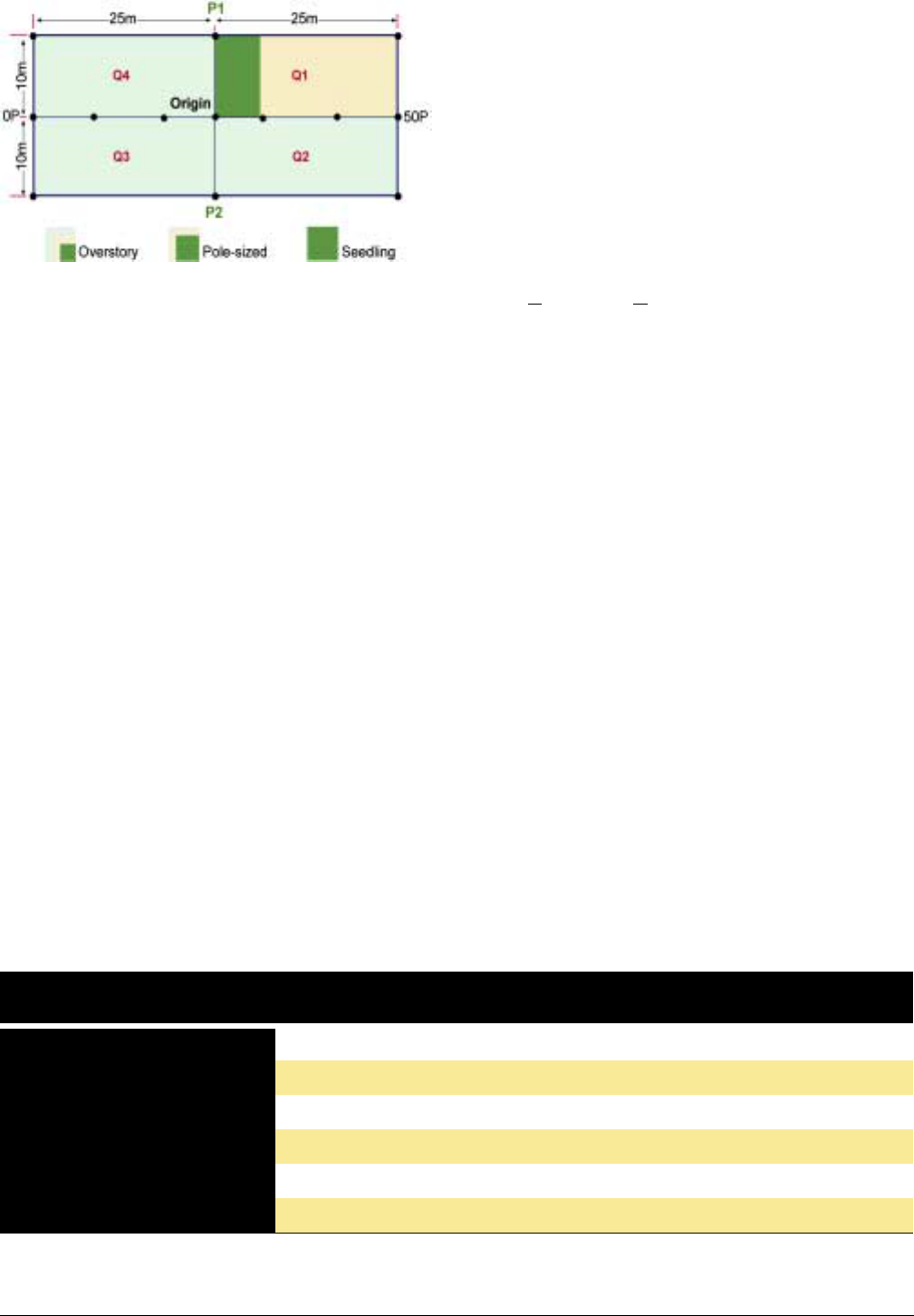
Figure 9. Suggested sampling areas for forest variables.

Plot Specifications

Suggested plot size and sampling locations vary for

each variable (see Figure 9 and Table 4). The plot sizes

and transect lengths in Table 4 are adequate for many

forest types, but revisions will in some cases be neces-

sary to reduce excessive data collection or to increase

data precision for a particular variable. These adjust-

ments may be particularly important when an objective

variable is sparsely distributed. All adjustments should

be done by resource and/or fire managers in consulta-

tion with a fire or vegetation ecologist.

Where variability is high, the calculated minimum sam-

ple size (number of plots, see page 49) may exceed 50.

There are five basic ways you can reduce this variabil-

ity:

1. Increase the area, number of sample points, or

transect lengths monitored for variables with high

variability throughout the monitoring type.

2. Change the shape of your sampling area.

3. Use another method to measure that variable (e.g.,

temporary plots are better than permanent plots at

monitoring changes in some annual plant popula-

tions).

4. Install a large number of monitoring plots.

Table 4. Suggested forest plot specifications, by variable.

5. Further stratify the monitoring types and create

additional sets of monitoring plots (see page 34 for

a discussion of splitting your monitoring types).

Locating and installing additional plots (needed for the

last two options) is very time-consuming; therefore, of

the options listed above, options one, two and three

are the preferred means of reducing variability.

Tree size classes

The suggested size class definitions for overstory

(DBH (diameter at breast height) >15 cm), pole-size

(DBH >2.5 cm and <15 cm), seedling (DBH <2.5 cm)

trees may work in some areas but not in others. If you

find that these definitions are not useful, and your park

ecologist, regional ecologist or fire effects monitoring

program manager agrees, you can redefine them. Be

sure to note any changes on the back of the Monitor-

ing type description sheet (FMH-4 in Appendix A).

Overstory trees

The 20 m × 50 m plot size may be unnecessarily large

for dense stands of overstory (DBH >15 cm) trees. In

these preburn situations, try using a pilot sampling

regime, such as the example displayed in Figure 10.

Where the overstory trees are very sparse (e.g., giant

sequoias, large mature trees) try enlarging (e.g., dou-

bling) the default sampling area during the pilot sam-

pling period. If only one species or size class is very

sparsely distributed, you may try larger sampling areas

for that species or size class alone during pilot sam-

pling. In this example, some plot sizes/shapes that you

could try for giant sequoia overstory trees might be: 20

m × 100 m or 40 m × 100 m; using 20 m × 50 m for

all other overstory species (not illustrated). In addition,

please read the Tip “Different Sizes and Shapes of

Sampling Areas” on page 47 and the Reminder “Con-

sistent Sampling Areas” on page 47.

Variable

Plot Size or

Transect Length Location

Overstory Trees

Plot: 20 m × 50 m (0.1 ha)

Plot: 10 m × 25 m (0.025 ha)

Plot: 5 m × 10 m (0.005 ha)

Transect: four, 50 ft each (200 ft)

Transect: two, 50 m each (100 m)

Plot: two, 1 m × 50 m (0.01 ha)

Quarters 1, 2, 3, 4

Quarter 1

Portion of Quarter 1

Quarters 1, 2, 3, 4

Outer portions of Quarters 1, 2, 3, 4

Pole-size Trees

Seedling Trees

Dead and Downed Fuels

Shrub and Herbaceous Layer

Shrub Density

Fire Monitoring Handbook 44

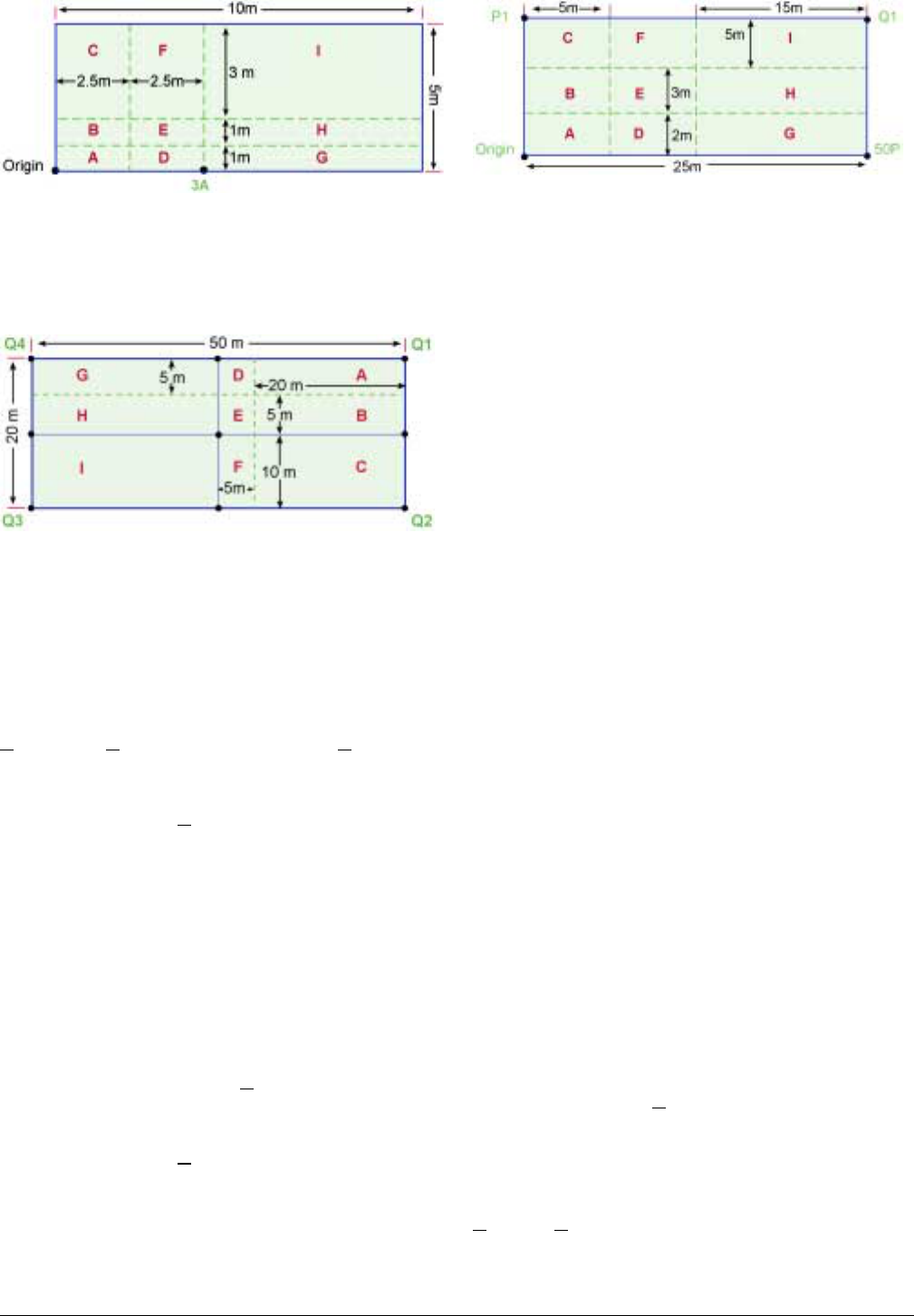
Figure 10. An example pilot sampling scenario for

extremely dense overstory or pole-sized trees.

Note: This example may not be suitable for your situation. The

shape and size combinations that can be tested here include: 2.5

× 1 m (A), 2 × 2.5 (A+B), 2.5 × 5 (ABC), 5 × 5 (A–F), 1 × 5 (A+D),

1 × 10 (A+D+G), 2 × 10 (A+D+G+B+E+H), 5 × 10 m (All).

Figure 11. An example pilot sampling scenario for sparse

pole-sized or seedling trees.

Note: This example may not be suitable for your situation. The

shape and size combinations that can be tested here include: 5 ×

20 m (A), 20 × 10 (A+B), 20 × 20 (ABC), 25 × 20 (A-F), 25 × 5

(A+D), 50 × 5 (A+D+G), 50 × 10 (A+D+G+B+E+H), 50 × 20 (All).

Pole-size trees

Where the preburn density of pole-size trees (DBH

>2.5 cm and <15 cm) is dense (averaging >50/250 m

2

(Q1)), try using a pilot sampling regime, such as the

example displayed in Figure 10. Where pole-size trees

are sparse (averaging <

20/250 m

2

), try using a pilot

sampling regime, such as the example displayed in

Figure 11. If only one species is sparsely distributed,

you may try larger sampling areas for that species alone

during pilot sampling. In addition, please read the Tip

“Different Sizes and Shapes of Sampling Areas” on

page 47 and the Reminder “Consistent Sampling

Areas” on page 47.

Seedling trees

Where the preburn density of seedling trees (DBH

<2.5 cm) is dense (averaging >50/50 m

2

(subset of

Q1)), try using a pilot sampling regime such as the

example displayed in Figure 12. Where seedling trees

are sparse (averaging <

20/50 m

2

), try using a pilot

sampling regime such as the example displayed in

Figure 11. In addition, please read the Tip “Different

Sizes and Shapes of Sampling Areas” on page 47 and

the Reminder “Consistent Sampling Areas” on page

47.

Figure 12. An example pilot sampling scenario for dense

seedling trees.

Note: This is only an example, and it may not be suitable for your

situation. The shape and size combinations that can be tested

here include: 2 × 5 m (A), 5 × 5 (A+B), 5 × 10 (A+B+C), 10 × 10

(A–F), 2 × 10 (A+D), 2 × 25 (A+D+G), 5 × 25 (A+D+G+B+E+H),

25 × 10 m (All).

Dead and downed fuels

During the pilot sampling period, on average, 75% of

the dead and downed sampling planes within a moni-

toring type should intercept a 3 in or larger diameter

log. If 3+ in intercepts are sparse (on average < 75%

of the sampling planes intersect a 3+ in intercept) try

extending the 50 ft sampling plane to 75 or 100 ft, or

longer, during pilot sampling. Designate intercepts that

lie along each section (e.g., 0–50, 50–75, and 75–100)

separately so that you can test the efficiency of each

length, and possibly shorten the plane length. Con-

versely, if 3+ in intercepts are dense (average number

of intercepts >30–40, e.g., heavy continuous slash), try

breaking up the 50 ft plane into 5 ft intervals starting at

15 ft, recording each interval separately so that you can

test the efficiency of each length. You can also modify

the sampling planes for 0–3 in intercepts. For further

details refer to Brown and others 1982. After pilot

sampling, indicate the final lengths of the sampling

planes on the back of the FMH-4. In addition, please

read the Reminder “Consistent Sampling Areas” on

page 47.

Shrub and herbaceous layer

You may need to try different lengths of point inter-

cept transects to intercept an adequate amount of

brush, grass and herbs during pilot sampling. In most

forested areas, 332 intercepts (two 50 m transects) may

be barely adequate since the shrub, forb, and grass ele-

ments are often sparse (an average of >55 and <110

hits/transect). Where the vegetation is extremely

sparse (an average of <

55 hits/transect) and one or

several of your herbaceous variables are objective vari-

ables, try reading the plot midline (0P to 50P; see

Figure 9, page 44) as a third transect during pilot sam-

pling. Where the vegetation is dense (an average of

>

110 and <140 hits/transect), monitor only one of the

50 m transects (monitor transect Q4–Q1 as a mini-

mum; see Figure 9, page 44). If the vegetation is

Chapter 4 n

nn

n Monitoring Program Design 45

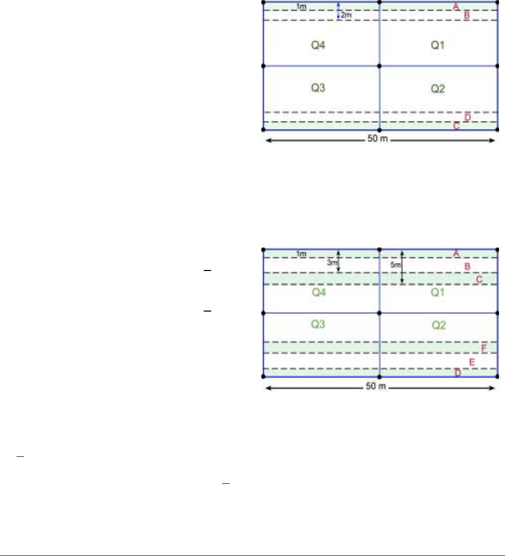
extremely dense (an average of >140 hits/transect),

try monitoring only 30 m of the 50 m transect (Q4–30

m). Note: During pilot sampling, you can easily test

the efficiency of shorter or fewer transects in each of

these scenarios by separating out those data. After

pilot sampling, indicate the final number and length of

the transect(s) on the back of the FMH-4. In addition,

please read the Reminder “Consistent Sampling Areas”

on page 47.

Basal cover—Because the cover of herbaceous spe-

cies and subshrubs can vary widely with climatic fluc-

tuations, it is often difficult to interpret changes in

their aerial cover. Such changes may be due to fire

management, weather, or a combination of both. Basal

cover is much less sensitive to climatic fluctuations and

can be a better trend indicator for species that are

suited to basal cover measurement (e.g., perennial

bunchgrasses). However, the aerial cover of most

woody shrubs does not tend to vary as much with cli-

matic fluctuations, and aerial cover is often used as an

indicator for these species.

If you do sample basal cover rather than aerial cover

(FMH default), place a note in the “Notes” section of

the Monitoring type description sheet, and follow the

directions on page 81. Be sure to use a line intercept

transect in your pilot sampling, as this is the traditional

method used to sample basal cover.

Species not intercepted but seen in the vicinity of

the herbaceous transect—Where the preburn num-

ber of herbaceous species is high—averaging >

50 spe-

cies/plot (using a 5 m belt), try using a pilot sampling

regime such as the example displayed in Figure 13. In

areas with low numbers of species (averaging <20 spe-

cies/plot, using a 5 m belt), try using a pilot sampling

regime such as the example displayed in Figure 14.

Once you have selected a belt width, use that width for

preburn and postburn measurements for all plots

within that monitoring type. In addition, please read

the Reminder “Consistent Sampling Areas” on page

47.

Shrub density

Where the preburn density of shrubs is dense (averag-

ing >50 individuals/plot, using a 1-m belt), try using a

pilot sampling regime such as the example displayed in

Figure 13. In areas with sparse shrubs (averaging <20

individuals/plot, using a 1-m belt), try using a pilot

sampling regime such as the example displayed in

Figure 14. In addition, please read the Tip “Different

Sizes and Shapes of Sampling Areas,” on page 47, and

the Reminder “Consistent Sampling Areas” on page

47.

In some shrub species, it can be hard to identify an

individual (see page 88 for more details). This is espe-

cially true for species that are capable of vegetative

reproduction, e.g., clonal or rhizomatous plants. In

these cases stem density (optional) can be used

instead of the number of individuals. Use the afore-

mentioned guidelines (replacing the counting of indi-

viduals with the counting of stems) to select the

appropriate sampling area for stem density.

Figure 13. An example pilot sampling scenario for dense

shrubs.

Note: This is only an example, and it may not be suitable for your

situation. The shape and size combinations that can be tested

here include: 1 × 5, 10 . . . 50 (A broken into 5 m intervals), 2 × 5,

10 . . . 50 (A+B broken into 5 m intervals). You would include C

and D if you use Q3–Q2 for herbaceous sampling during the pilot

sampling period.

Figure 14. An example pilot sampling scenario for sparse

shrubs.

Note: This is only an example, and it may not be suitable for your

situation. The shape and size combinations that can be tested

here include: 1 × 5, 10 . . . 50 (A broken into 5 m intervals), 3 × 5,

10 . . . 50 (A+B broken into 5 m intervals), 5 × 5, 10 . . . 50

(A+B+C broken into 5 m intervals). You would include D, E and F

if you use Q3-Q2 for herbaceous sampling during the pilot

sampling period.

Fire Monitoring Handbook 46

Different Sizes and Shapes

of Sampling Areas

To decide which sizes and shapes of sampling areas to

try, observe the distribution of plants in the field. Ask

yourself which sizes and shapes, on average, would

include one or more of the largest individuals or

patches, while minimizing the number of empty quad-

rats. Be sure to try and include long and thin rectangles

(0.25 × 4 m instead of 1 × 1 m), and/or shapes that are

proportional to your other sampling areas, e.g., 20 × 50

m for overstory trees, 10 × 25 m for pole size trees,

and 5 × 12.5 m for seedling trees. Both have been

shown to have statistical advantages. In addition, if

only one species or size class is sparsely (or densely)

distributed, you may try larger (or smaller) sampling

areas for that species or size class alone during pilot

sampling.

Consistent Sampling Areas

You must have consistent sampling areas for each vari-

able within a monitoring type. In other words, keep the

length or size/shape of all transects or areas where you

collect data (e.g., fuels, shrub density, herbaceous cover,

overstory, pole-size and seedling tree density) the same

for a given variable throughout a monitoring type. See

page 88 (shrub seedlings) and 102 (tree seedlings) for

the only exceptions to this rule. Note: After pilot sam-

pling, indicate the final shape and size of the sampling

area on the back of the FMH-4.

Optional Variables

Diameter at root crown for woodland species

Woodland species such as juniper, pinyon pine, some

maples and oaks commonly have multiple stems and

are often extremely variable in form. For these species,

diameter at root crown (DRC) is a more meaningful

measurement than DBH (USDA Forest Service 1997).

Indicate each species that you will measure using DRC

in the “Notes” section of the Monitoring type descrip-

tion sheet (FMH-4). Pilot sampling procedures are the

same as for overstory and pole-size trees: see above.

Herbaceous density

Where the preburn density of forbs and grasses is

dense (averaging >50 individuals/plot, using 1 m

2

frames), try a pilot sampling regime using smaller

frames of differing shapes. You may also find that you

are sampling too many frames. In preburn situations

where forbs and grasses are sparse (averaging <20

individuals/plot, using 1 m

2

frames), try a pilot sam-

pling regime using larger frames of differing shapes, or

try using a pilot sampling regime such as the examples

displayed in Figure 13 and 14.

Biomass

Estimate preburn biomass (tons/acre) when smoke

management is a specific concern, or hazard fuel

reduction is the primary burn objective. This hand-

book mentions three methods of measuring biomass:

the dead and down fuel methods discussed above (for-

est), estimation (brush, page 89); and clipping (grass-

land, page 90). To determine appropriate plot size for

estimation, see Mueller-Dombois and Ellenberg 1974.

Note: Use the pilot sampling process to choose the

most efficient sampling areas.

To determine the appropriate quadrat size for clipping,

see Chambers and Brown 1983. There are several

other methods for estimating biomass: relative weight,

height-weight curves, photo keys, capacitance meters,

remote sensing, and double sampling. For an excellent

list of references, see Elzinga and Evenden 1997 under

the keyword biomass, or review the references on page

237 in Appendix G. Once you choose a methodology,

write a “handbook” for your field protocols so that

others can collect these data exactly the same way you

do. Refer to this “handbook” in the “Notes” section of

the FMH-4 for that monitoring type.

Percent dead brush

To develop a custom fuel model for BEHAVE or

other fire behavior predictions, estimate the preburn

percent dead brush with one of the following tech-

niques: onsite visual estimation, estimation based upon

a photo series, or direct measurement of the live-dead

ratio. Again, once you choose a methodology, write a

“handbook” for your field protocols so that others can

collect these data exactly the same way you do. Refer to

this “handbook” in the “Notes” section of the FMH-4

for that monitoring type.

DEVIATIONS OR ADDITIONAL

PROTOCOLS

Rarely will a sampling design work smoothly in the

field; you will often find that modifications are needed.

You may also find that in some situations the methods

in this handbook will not work to sample your ecologi-

cal attribute of interest. If this is the case, refer to a

reputable vegetation monitoring source such as Bon-

Chapter 4 n

nn

n Monitoring Program Design 47

ham 1989, or to a bibliography of vegetation monitor-

ing references such as Elzinga and Evenden 1997.

The FMH software (Sydoriak 2001) that accompanies

this handbook is designed for the protocols in this

handbook, and facilitates data storage and analysis. In

some cases, where other methods are used, you will

need to set up an alternative database and perform

analyses with a commercial statistical software pack-

age. It is important to document all deviations from

the standard protocols used in this handbook, no mat-

ter how insignificant they may seem. These notes are

critical links for the people who follow you, and will

ensure that the appropriate protocols are continued

until the end of the project. Reference any additional

protocols in the “Notes” section of the Monitoring

type description sheet (FMH-4 in Appendix A), and

describe them completely in your monitoring plan

(Appendix F).

CONSIDERATIONS PRIOR TO FURTHER

PLOT INSTALLATION

After you have completed your pilot sampling, answer

these questions:

• Are the sampling units for each protocol a reason-

able size for the average number of plants?

• Did you choose the most appropriate vegetation

attribute–one that is easy to measure and the most

sensitive to change–that will meet your monitor-

ing objectives?

• Will you and your successors be able to relocate

your monitoring plots in future years using the

proposed documentation method?

• Is the time you allotted for the field portion of the

monitoring adequate?

• Is the time you allotted for the data management

portion of the monitoring program adequate?

(This typically takes 25-40% of the time required

for a monitoring program). Do you have ready

access to a computer for data entry and analysis?

On average, do you have a small number of tran-

scription errors?

• Will it be easy for monitors to avoid seriously

trampling vegetation? (If not, is this acceptable?)

• Do monitors find it difficult to accurately position

a tape because of dense growth?

• Are your field personnel skilled, with only a minor

need for additional training?

• Did you meet your precision and power objec-

tives? Does the amount of change you have cho-

sen for your minimum detectable change seem

realistic? Does the time period for this change

seem realistic?

SAMPLING DESIGN ALTERNATIVES

If you answered no to one or more of the above ques-

tions, consider adjusting your monitoring design. Here

are some alternatives to consider:

Start over from the beginning of the process—

Revisit your monitoring objective with the realization

that it is not cost-effective to monitor that objective

with a reasonable level of statistical precision or power.

Accept lower confidence levels—Ask yourself

whether you would find a lower confidence level

acceptable. It can be very costly to set up a monitoring

program with a 95% confidence of detecting a change.

However, you might find it quite possible to use your

available resources to monitor at a 80% confidence

level. Look at the results from your pilot study and ask

yourself if you could be comfortable with a higher

error rate.

Request more resources for monitoring—You can

try to get additional funding from other sources, such

as grants or park-wide funding. Also, consider using

interns, students, and volunteers to supplement your

staff.

Reconsider the scale of the study—Choose to sam-

ple a smaller subsection of your monitoring type. Note

that this may diminish the statistical applicability of

your results.

Reconsider your sampling design—Adjust the

shape or size of the sampling area for a troublesome

variable. For example, based on the pilot study, create a

different size and/or shape for the brush sampling

area.

Look for data entry or data collection errors—

Occasionally, an appropriate sampling design may

combine with a sufficient number of data errors to

give the appearance of a flawed sampling design.

Check the data collected during the pilot study for field

errors; also check for data entry errors. Simple errors

can significantly skew calculations such as the standard

deviation. See the “Verifying Results” section on page

131 for more details.

Fire Monitoring Handbook 48

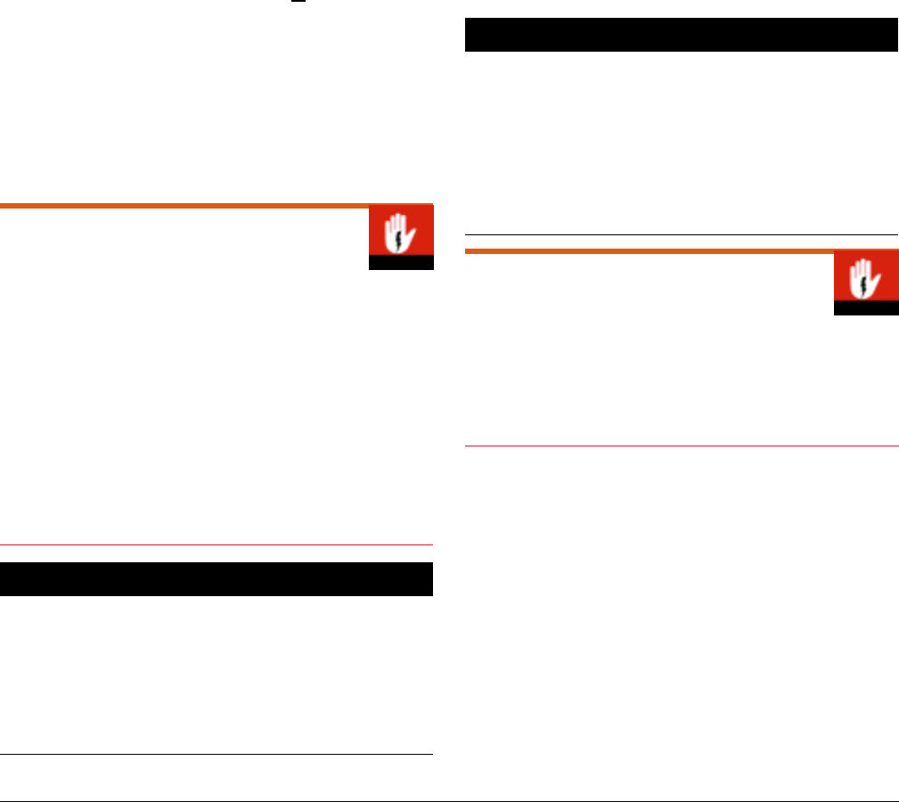
CALCULATING MINIMUM SAMPLE SIZE

The minimum sample size for your monitoring design

is the number of plots needed (based on your initial

10-plot sample mean and variability to provide results

with your chosen degree of certainty (see pages 23 and

122). An estimate of the variability found for a particu-

lar objective variable gives an idea of the number of

plots needed to obtain a reasonable estimate of the

population mean with the desired confidence level and

precision (see page 27).

To calculate the initial minimum sample size, you need

the following inputs:

• Mean and standard deviation of the sample—

data from the 10 initial plots in each monitoring

type are used as estimates of the mean and vari-

ability for each objective variable

• Desired level of certainty—confidence level (80,

90, or 95%) and precision level (<

25% of the

mean) from your monitoring objective

Once you have these inputs, you can use the formula

on page 216 (Appendix D) to calculate the minimum

sample size (number of plots) needed to provide the

chosen levels of certainty for estimating the mean(s) of

the objective variable(s) in a monitoring type.

Minimum Sample Size

Keep in mind that the minimum sample size only

applies to the monitoring variable that is used in the

calculation(s), not to all of the variables measured

within the plot. See page 217 for an example of calcu-

lating minimum sample size for each type of manage-

ment objective—condition and change.

Calculate the minimum sample for each objective vari-

able in a monitoring type, then use the largest sample

size when installing plots.

Example:

Two objective variables in a monitoring type are total

percent cover of live shrub species and native peren-

nial relative cover. The calculated minimum sample

size is 17 plots for total shrub percent cover and 15

plots for native perennial relative cover; 17 plots

should be installed.

If the minimum sample size calculated is high (>30

plots) based on the initial 10 plots, install several more

plots (2–5) and then recalculate the minimum sample

size. If the minimum sample size continues to be high,

refer to the advice on page 44. The monitoring type

may be too broad or the method used to measure the

monitoring variable may not be appropriate. As always,

consult with your regional fire effects program coordi-

nator for assistance if needed.

If the minimum sample size is very low, you may be

able to increase the degree of certainty in the sample

simply by installing a few more plots. Only add addi-

tional plots if it will not require a great deal of extra

time and effort and if it will provide a useful increase

in the certainty of the results. Note: Increase the con-

fidence level before increasing the precision level; in

other words, be more confident in your results before

attempting to be within a smaller percentage of the

estimated true population value.

Example:

Only ten plots are needed to be 80% confident of

being within 25% of the estimated true population

mean for the density of tamarisk (Tamarix ramosis-

sima). The resources to install a few more plots are

available; therefore, recalculate the minimum sample

size with a 90 or 95% confidence level to see if the

resulting number of additional plots is practical.

Confidence Level and Precision

Always choose the confidence level and precision

desired BEFORE performing the minimum sample

size calculation. It is not appropriate to run all possibil-

ities and choose the preferred minimum sample size!

Chapter 4 n

nn

n Monitoring Program Design 49

Change Over Time

Your management objectives define either the amount

of change or a postburn condition desired for a moni-

toring variable. Ideally, you should calculate the mini-

mum sample size needed to detect the desired

minimum amount of detectable change or postburn

condition. In order to do this, however, you need an

estimate of the mean and variability of the monitoring

variable for both preburn and postburn conditions.

Since managers must design the monitoring program

before burning, your initial minimum sample size cal-

culations must be based only on the preburn data.

Recalculate Minimum Sample Size

The initial minimum sample size calculation is per-

formed on the preburn data so that a sufficient num-

ber of plots can be distributed in areas before they are

burned. Since the management objectives usually

involve assessing postburn conditions, you should

recalculate the minimum sample size for the appropri-

ate postburn time interval when it is reached. For

change objectives, a separate formula is used to deter-

mine the number of plots needed to detect the mini-

mum amount of change stated in the objective (see

page 217).

Minimum Sample Size for

Minimum Detectable Change

This formula is a critical new addition to this hand-

book. For change objectives, calculate the minimum

sample size for the minimum detectable change you

desire before you fully evaluate whether you have met

your objectives. See pages 124 and 217.

MONITORING DESIGN PROBLEMS

Small Areas

Some monitoring types may occupy areas that are

small as compared to the majority of the monitoring

types in your park. This monitoring program is

designed to support the monitoring of the monitoring

types that constitute the most significant amount of

acreage that is being burned in your park. However,

you might consider monitoring small areas if they con-

tain species of management concern. In these cases,

managers might consider using a sampling design bet-

ter suited to a smaller scale or species-specific moni-

toring, which you should have reviewed by your

regional ecologist and fire effects monitoring specialist.

Gradient Monitoring

In many instances your objectives will require monitor-

ing in vegetation that does not occur in one discrete

unit or in a homogeneous vegetation type. This will be

the case when you monitor ecotones, or other areas of

encroachment, e.g., grasslands being invaded by

shrubs, trees, and/or non-native plant species.

No single set of protocols will serve all monitoring

programs. This handbook is not intended to be a

definitive “how-to” guide on monitoring. The proto-

cols of this handbook are designed to monitor trends

in a relatively homogeneous complex of vegetation—a

monitoring type. They are not specifically designed to

measure changes across a gradient.

With this in mind, you can make modifications to the

protocols of this handbook to monitor changes across

a gradient or movement of a transition zone. It is

important to determine the variable of concern and

direction you wish to take the system with the use of

fire.

Note: Before you make these modifications, find out

if other park units have similar objectives. Others may

have developed modifications to the protocols in this

handbook, or use alternative sampling methods that

may be useful to you.

Species Difficult to Monitor

Ephemeral annuals or annuals with long-lived

seed banks

If your monitoring objectives concern annual plants

that appear only once every few years or decades, or

that have long-lived seed banks, short-term data may

misrepresent the species’ presence in the ecosystem.

Interpretations of field measurements on annual spe-

cies are confounded by the yearly variability of their

distribution and abundance. In such situations, an

alternative may be to monitor the critical elements of

the habitat of this species, e.g., changes in the type and

amount of disturbance (fire, flood, trampling, etc.),

and changes in community composition and structure.

When dealing with such annuals, it is extremely helpful

to know what factors promote or infringe upon the

vitality of the species.

Fire Monitoring Handbook 50

Example:

you erase data and remove any rebar, consult with both

fire and resource management personnel.

A park with chaparral plant communities seeks to

manage the postfire species seed bank by burning at

Professional Input and Quality

an interval that is less than the average seed longevity

Control

(which is largely unknown for the majority of the

species in the seed bank). Managers are confident

that a return interval of 50–100 years will keep this

seed bank replenished. The majority of species that

appear postburn are annuals, and so will have an

unpredictable distribution pattern for several years

postburn. Since monitoring species with an unpre-

dictable distribution pattern can be cost prohibitive,

managers have decided to monitor the factors that

affect the species distribution: gaps in canopy cover,

and the frequency and intensity of soil disturbances.

Extremely long-lived plants

Plants that live a long time pose an opposite problem;

variation in population size is very long-term, so

change is difficult to measure. Reproduction and/or

seedling establishment can be a rare event (although

for some long-lived species, seedlings are dynamic and

very sensitive to adverse change). Once again, moni-

toring changes in the plants’ habitat may be more

appropriate than measuring the plants themselves.

Anticipated dramatic increases in postburn

density

The seed banks of some species may germinate pro-

fusely following a burn. Rather than count thousands

of seedlings, it may be more efficient to subsample the

plot during temporary high density periods. See pages

88 and 102 for details.

Monitoring Type Description Quality Control

Ensuring consistency in the definition of a monitoring

type—and thus in the establishment of plots—is criti-

cal to the accuracy of a monitoring program. Often,

plots are established before the creation of monitoring

type descriptions. In addition, if Monitoring type

description sheets are unclear or vague, monitors may

establish plots that should be rejected.

All managers can benefit from reviewing some or all of

their plots to ensure that each plot belongs within the

designated monitoring type. Any plots that should be

rejected can be erased from the database and the plot

markers (rebar) removed, and the respective folders

discarded, unless resource management has further use

for these plots. Rejected plots may be useful for train-

ing purposes or resource management needs. Before

It is very important that the monitoring program be

designed with enough professional input to reduce

problems associated with improper data collection.

Equally important is the provision of quality control

during the data collection process. Ignoring either of

these critical elements could mean bad or useless

results. If poor design or quality are problems, the first

monitoring protocol adjustment is to start over and

ensure that proper monitoring protocols are applied

throughout the data collection period the next time

around.

A common problem is inadequate attention to the

design and documentation of the monitoring proto-

cols and/or insufficient supervision of the data collec-

tion team. The fire effects monitors may make poor

decisions, especially if their decision makes their job

easier (e.g., switching quadrats because of the large

number of trees present in the designated quadrat).

Thoughtless data collection can lead to the omission

of whole categories of variables. Alternatively, more

data may be collected than prescribed in the sampling

design, wasting valuable time and energy. Extra work is

then required to sort out which datasets are valid and

which components of these datasets are not compara-

ble. The key is to prevent problems by properly

designing, supervising, and periodically checking the

monitoring protocols used.

Decide and document when and how monitoring pro-

tocols will be adjusted, and who is responsible. No

matter how carefully you design a monitoring program

or how expertly it is carried out, data collection prob-

lems will arise and monitoring protocols will have to

be adjusted. Such adjustments should be made not by

the field technicians, but by the program managers and

ecologists. The more managers are involved in the data

collection process, the sooner they will recognize pro-

tocol problems.

Establish a decision-action trail by documenting proto-

col changes. All changes to established monitoring

protocols must be documented so that the changes can

be replicated every time you remeasure your plots. The

following tips will help you document your monitoring

Chapter 4 n

nn

n Monitoring Program Design 51

protocol, make any necessary changes, and ensure its

consistent use:

• Educate everyone involved about the importance

of strictly adhering to monitoring protocols.

• Establish a process for changing protocols based

on field work and analytic results, with input from

your data collectors.

• Consult with your regional fire effects program

manager on the protocols, as well as on any

changes.

• Diligently record all protocol changes.

• Mark all changes in colored ink. Label changes in

clear bright colors, or place them collectively on

bright colored paper.

• Enter any protocol deviation into a database com-

ment field for that plot or monitoring type.

• Communicate, as often as possible, with all inter-

ested parties.

• Put the monitoring protocols in writing in your

Monitoring type description sheet (FMH-4) and

your monitoring plan (Appendix F), and place

them in the plot folder. Make sure that originals

are never lost and that copies are always in the

possession of the data collectors.

CONTROL PLOTS

It is not currently national policy to use fire funds

to pay for the installation of control plots (see Glos-

sary), but control plots can be necessary to evaluate

whether specific management objectives are met.

Depending on your objectives, it may be important to

make observations and collect data outside of pre-

scribed burned areas.

Frequently, control plots are not considered until post-

burn observations indicate their need. It is often

appropriate to establish control plots after the burn

when you need to address a specific question. In the

case of wildland fires, some managers may wish to

establish control plots outside the burn perimeter dur-

ing the field season following the fire.

When control plots are established to measure specific

variables, use methods and certainty levels comparable

to their preburn counterparts. Decisions about when

and how to install control plots will require consulta-

tion with an ecologist, statistician, or other subject

matter expert. In many cases the implementation of a

formal research project may be more appropriate.

When deciding not to install control plots, the park

manager recognizes either that an adequate fire effects

information base is available to start or continue a

burn program, or that ongoing research programs are

adequate to address management concerns.

Control Plots

Comparing your data with those from other parks that

have similar monitoring types, or from other types of

studies internal or external to your park may eliminate

the need for you to set up control plots. Consult an

ecologist, statistician and/or regional fire effects moni-

toring specialist for further assistance.

Short-term Change Control Plots

Control plots are often necessary to determine

whether the prescribed fire program caused a particu-

lar short-term effect.

Example:

A burn block area has been invaded to a small extent

by non-native species. Non-native species have been

increasing throughout the region for the last 20 years,

and the park manager does not want to worsen the

problem by using prescribed fire. In fact, one of the

management objectives is to reduce the mean non-

native species percent cover by 20–60% within two

years of the burn. You know that your prescription

can meet your other management objectives, but you

suspect that the slow and incessant march of non-

native plants could be accelerated by the prescribed

fire.

In this example, and in many situations involving non-

native species, it is important to set up control plots to

test whether the result observed (a change in non-

native species percent cover) in the prescribed fire area

is attributable to fire or to another factor, such as cli-

matic change, moisture regimes, or grazing.

Long-term Change Control Plots

Establishing control plots for evaluating long-term

change is helpful for testing specific hypotheses com-

paring non-treatment effects (areas not treated with

prescribed fire) with treatment or treatment-plus-time

effects.

Fire Monitoring Handbook 52

Example:

A shrubland is burned every 20 years to reduce the

fuel hazard. The natural fire return interval is esti-

mated to be 50 years. After 100 years of fuels treat-

ment by fire, it is hypothesized that a difference in

composition and density exists between those stands

that have been burned every 20 years and the unman-

aged stand.

If you wish to evaluate control plots for long-term

change, you will need to consult a competent research

scientist or fire ecologist to ensure adequate research

design and execution.

DEALING WITH BURNING PROBLEMS

Burning the Prescribed Fire Units

Consistency of treatment is essential to ensure accurate

monitoring data. All monitoring plots within a sample

must be burned under the same prescription. Similarly,

burn units with monitoring plots must be treated the

same as units without monitoring plots. If a burn unit

is ignited but the monitoring plots contained within it

do not burn, data on those monitoring plots are still a

valid part of the sample database. Avoid biasing results

by igniting a monitoring plot prior to igniting the sur-

rounding area, or igniting the plots at a later time

because they did not burn initially (unless, of course,

the burn prescription calls for this action). All ignition

personnel should be informed that they need to ignite

every burn unit as if the plots do not exist, so that

burning patterns will not be biased.

Partially burned plots

Fire rarely spreads uniformly across a fuel bed.

Unburned patches are frequently part of the fire

regime and should not be of concern as long as the

plot was burned similarly to the remainder of the burn

unit. A partially burned plot, if burned within prescrip-

tion, should be considered part of the database.

Plot Burning Off-Schedule

Monitoring plots may reburn because of unplanned

ignitions (natural or human-caused) or short burn pre-

scription intervals. Other plots may be burned at a

time different from the rest of the unit. As a manager,

you need to decide when to eliminate such plots from

the sample, and whether to reinitialize the monitoring

schedule for that plot.

Unplanned ignitions

Unplanned ignitions that are permitted to burn

because they meet the prescription criteria of a pre-

scribed fire regime (and essentially replace a prescribed

ignition) will be treated as a component of the man-

aged fire regime. Monitoring schedules for plots in

such areas should not be altered. However, it is recog-

nized that considerable variation may enter the system

and affect index parameters if many monitoring plots

burn more frequently than prescribed. Managers will

have to keep this in mind and make evaluation adjust-

ments when examining results. In any case, it is essen-

tial to record the data collected from any unplanned

ignition in appropriate plot database files. Fire behav-

ior and weather data should also be included.

Plot burns at different time than the burn unit

Occasionally a plot may burn before or after the

majority of the burn unit. Are the data from this plot

still valid? That depends. If the area surrounding and

including the plot is burned within prescription using

the same ignition techniques, the plot data should be

valid. However, the plot should not be allowed to burn

off-schedule, i.e., more often or less often than the

burn prescription calls for.

Short fire intervals

In this situation, you will generally want to monitor the

responses from the prescribed fire regime rather than

from a single fire, as the changes caused by a single fire

are usually not as important. When the intervals

between prescribed fires are very short (one to two

years), resulting in frequent burn repetitions, conduct

immediate postburn (within two months postburn),

and year-1 postburn monitoring on the first and subse-

quent burns until you can predict responses (if year-1

postburn monitoring is not possible, you can substi-

tute measurements from the next field season).

Choose the most representative time(s) to track the

changes you would like to detect (e.g., six months after

every burn combined with monitoring on a five-year

rotation), regardless of how often each plot burns.

If the fire interval is longer than two years, conduct

immediate postburn (within two months postburn),

year-1, year-2 and year-5 (if possible) postburn moni-

toring on the first and subsequent burns until you can

predict responses. Choose the most representative

time(s) between burns. In some situations, pre- and

immediate postburn monitoring will be your best

choice. For example, add a “preburn” measurement

for each subsequent burn, e.g., year-2 for a two-year

return interval, year-3 for a three-year return interval

or year-4 for a four-year return interval.

Chapter 4 n

nn

n Monitoring Program Design 53

Plot burned out-of-prescription

Eliminate monitoring plots from the sample database

if they are burned by planned or unplanned fires that

exceed the ecological parameters of the management

prescription. Keep in mind that you may want to con-

tinue to monitor these plots in order to gain informa-

tion about the response from a different prescription.

Fire Monitoring Handbook 54

3

Vegetation Monitoring Protocols

5

Vegetation Monitoring Protocols

“It takes less time to do a thing right than it does to explain why you did it wrong.”

—Henry Wadsworth Longfellow

As indicated in Chapter 4, for short-term and long-

term monitoring (levels 3 and 4), you will monitor Rec-

ommended Standard (RS) variables by sampling

according to a standardized design. When combined,

monitoring plots form a sample for each monitoring

type, with or without control plots. This chapter details

variables and procedures for establishing monitoring

plots, and for collecting and recording data from them.

Note: This handbook addresses most common situa-

tions; special concerns may require customized meth-

ods.

This handbook establishes RS variables for grassland,

brush, and forest plot types. The monitoring variables

sampled for each type are cumulative, with increasingly

complex plot types (grassland to brush to forest)

including variables in addition to those sampled on the

simpler types (see Table 3, page 42).

The procedures described for monitoring RS variables

require the use of standardized forms to record data;

these are provided in Appendix A. Methods and data

collection forms also are provided for most of the

optional monitoring variables.

Establishing a plot network for a given monitoring

type is a three-phase process. As discussed in Chapter

4, this process begins with the installation of ten pilot

sampling plots. Once these plots are installed, mini-

mum plot calculations and projections are conducted;

the process ends with the installation of the balance of

plots required by the minimum plot analyses. This sec-

tion outlines the methods that you will follow for the

establishment of all plots.

METHODOLOGY CHANGES

Some sampling methods described here are signifi-

cantly different from methods presented in previous

versions of this handbook. In a monitoring type with

previously burned plots, exercise extreme caution

before changing your methods; in most cases meth-

ods should not be changed. If you do intend to

change monitoring methodologies, then monitor using

both methods for a minimum of two plot visits (for

each plot affected), or until you can establish a corre-

lation between the different protocols. If no plots have

burned within this time period, revisit all plots in the

type and collect data according to the new protocol.

Additional procedures for handling the switch-over

can be found in “warning” boxes on specific topics,

e.g., crown position (page 96) and DRC (page 98).

MONITORING SCHEDULE

Sample during the phenological peak of the season

(flowering, as opposed to green-up, transition or dor-

mant) in which the plants can most easily be identified

and when biomass is greatest. This may occur in the

spring in low-lying areas with warm climates, and as

late as late summer for alpine regions; the peak sam-

pling season may occur twice in one year in some

areas, e.g., those with summer “monsoons.” The actual

date of this phenological stage will vary from year to

year, depending on climatic conditions. Schedule your

sampling to minimize seasonal variation among visits.

From year to year, base your sampling schedule on the

original date of establishment; however, you may have

to change the date of the visit due to seasonal irregu-

larities such as prolonged snow cover or an early, warm

spring. Except immediate postburn, conduct all visits

when phenology is comparable for the most ephem-

eral species recorded in the initial survey. Take notes

on the phenological state of the plants at each visit so

that you can consider whether these differences are the

result of burning or due to other factors such as

weather variations. It is recommended that you

monitor all plots at the intervals discussed below.

Plot Installation

To prepare for plot installation you will need the fol-

lowing: a five-year burn plan, delineated areas for plot

installation, and randomly selected plot location

points. After you have completed your pilot sampling

and you have ten plots in a single monitoring type, you

can then analyze the monitoring variables to determine

their variability within your sample. Use this informa-

tion to determine how many plots are required to

meet the specified confidence and precision levels

(see page 49 for details). The additional plots should

55

then be installed in the same manner as the initial ten

plots (using the restricted random method, page 59).

Ideally, all plots should be installed before any of the

available plot area has been burned, otherwise the total

area available for additional plot installation will be

reduced, which could result in a bias in the data. If it is

not possible to install all plots before burning any of

the monitoring type, then install your initial group of

plots in the first units to be burned.

Plot Location and Burn Units

• Monitoring types should not be directly associated

with individual burn units. Use the sample

approach, which states that random plot location

points shall be installed in all areas within a particu-

lar monitoring type that are scheduled to be burned

in the next five years. Plot location points should be

randomly selected within a monitoring type, not a

burn unit.

• Choose your burn units and write your monitoring

type descriptions before you install any plots.

• Note that plots do not need to be placed in every

burn unit.

Limited Amount of the Monitoring

Type Available for Burning

If the amount of the monitoring type available for

burning is limited, plan carefully. Check the burn

schedule relative to your potential plots, and be sure to

include plots in all representative areas using restricted

randomization. Remember, when fire managers burn a

section of monitoring type before you install the mini-

mum number of plots, that section can no longer be

included in your sample, i.e., you cannot install any

additional plots in that section.

Preburn

Establish plots during the time of year in which you

can identify the greatest number of species (particu-

larly the most ephemeral), so that you can obtain the

most complete species composition data within a

monitoring type. Ideally, the plots are burned the same

year in which the preburn data are collected. If more

than two years have passed since establishment or the

last data collection, remeasure variables prior to burn

treatment.

During Burn

Make fire behavior observations in an area near to, but

not necessarily at, each plot, and in the same fuel

model and vegetation type as that in which the plot is

located.

Immediate Postburn

Assess burn severity as soon as possible after the duff

stops smoldering. Assess all other RS measurements

between two weeks and two months after the burn

treatment.

Postburn

The recommended schedule for re-measuring plots

that have burned is one, two, five and 10 years post-

burn. After 10 years, continue the monitoring at 10-

year intervals either until each unit is placed within an

area approved for fire use (formerly PNF zones), or

the area is burned again. If the area is burned again,

the monitoring cycle begins again. For the monitoring

schedule for monitoring types that will be burned fre-

quently, or for situations in which plots should other-

wise be read on a different schedule, see page 53.

Recommended Standard (RS) variables to be moni-

tored pre- and postburn are listed in Tables 5–7.

In most cases, collect the preburn and postburn

(except immediate postburn) data during the pheno-

logical peak (see page 55). For example, if you con-

duct a preburn visit in July 2001, and the plot burns in

October 2001, the year-1 data should be collected at

the phenological peak in or near July 2002. If the plots

are burned in the season preceding the phenological

peak, collect postburn data a full year later. For exam-

ple, if you read a preburn plot in August of 2002, and

that plot burns in March 2003, collect the year-1 data

in or near August 2004. In moist areas, where vegeta-

tion recovers quickly, it may be desirable to collect data

sooner than year-1. In that case, code that data collec-

tion period as an interim data collection visit (e.g., six

months) and collect this information in addition to

your other plot visits.

Fire Monitoring Handbook 56

- -

Table 5. Grassland plot RS variables to be monitored pre- and postburn.

RS Variables PRE Immediate Postburn Year-1+

Herbaceous Cover (FMH-16)

n

Optional

n

Burn Severity (FMH-22)

n

Photographs (FMH-23)

n n

Table 6. Brush plot RS variables to be monitored pre- and postburn.

RS Variables PRE Immediate Postburn Year-1+

Herbaceous Cover (FMH-16)

n

Optional

n

Shrub Density (FMH-17)

n

Optional

n

Burn Severity (FMH-22)

n

Photographs (FMH-23)

n n

Table 7. Forest plot RS variables to be monitored pre- and postburn.

RS Variables Data Sheet(s) PRE Immediate

Postburn

Year 1 Year 2+

Tree Density Overstory (FMH-8)

n n n

Pole (FMH-9)

n

Optional

n n

Seedling (FMH-10)

n n n n

DBH/DRC Overstory (FMH-8)

n

Optional

n

Pole (FMH-9)

n

Optional

n

Live/ Dead Overstory (FMH-8, FMH-20)

n n n n

Pole (FMH-9, FMH-20)

n

Optional

n n

Fuel Load (FMH-19)

n n n n

Herbaceous/Shrub Cover (FMH-15 or FMH-16)

n

Optional

n n

Density (FMH-17)

n

Optional

n n

Burn Severity (FMH-21 or FMH-22)

n

Photographs (FMH-23)

n n n n

% Crown Scorch Overstory (FMH-20)

n

Pole (FMH-20) Optional

Scorch Height Overstory (FMH-20)

n

Pole (FMH-20) Optional

Char Height Overstory (FMH-20) Optional

Pole (FMH-20) Optional

Chapter 5 n

nn

n Vegetation Monitoring Protocols 57

DBH Remeasurement

Previous versions of the Fire Monitoring Handbook

stated that DBH should be measured at every plot visit

with the exception of immediate postburn. The new

recommendation is to skip this measurement at the

year-1 visit and to remeasure it at the year-2 visit. DBH

is a fairly gross measure for tracking tree growth; in

most cases the most important reason for tracking tree

growth is to assign the tree to a size class, and preburn

and year-2 measurements are usually sufficient for this.

If you feel that you have good justification for measur-

ing DBH at year-1, then by all means measure it!

Fire Monitoring Handbook 58

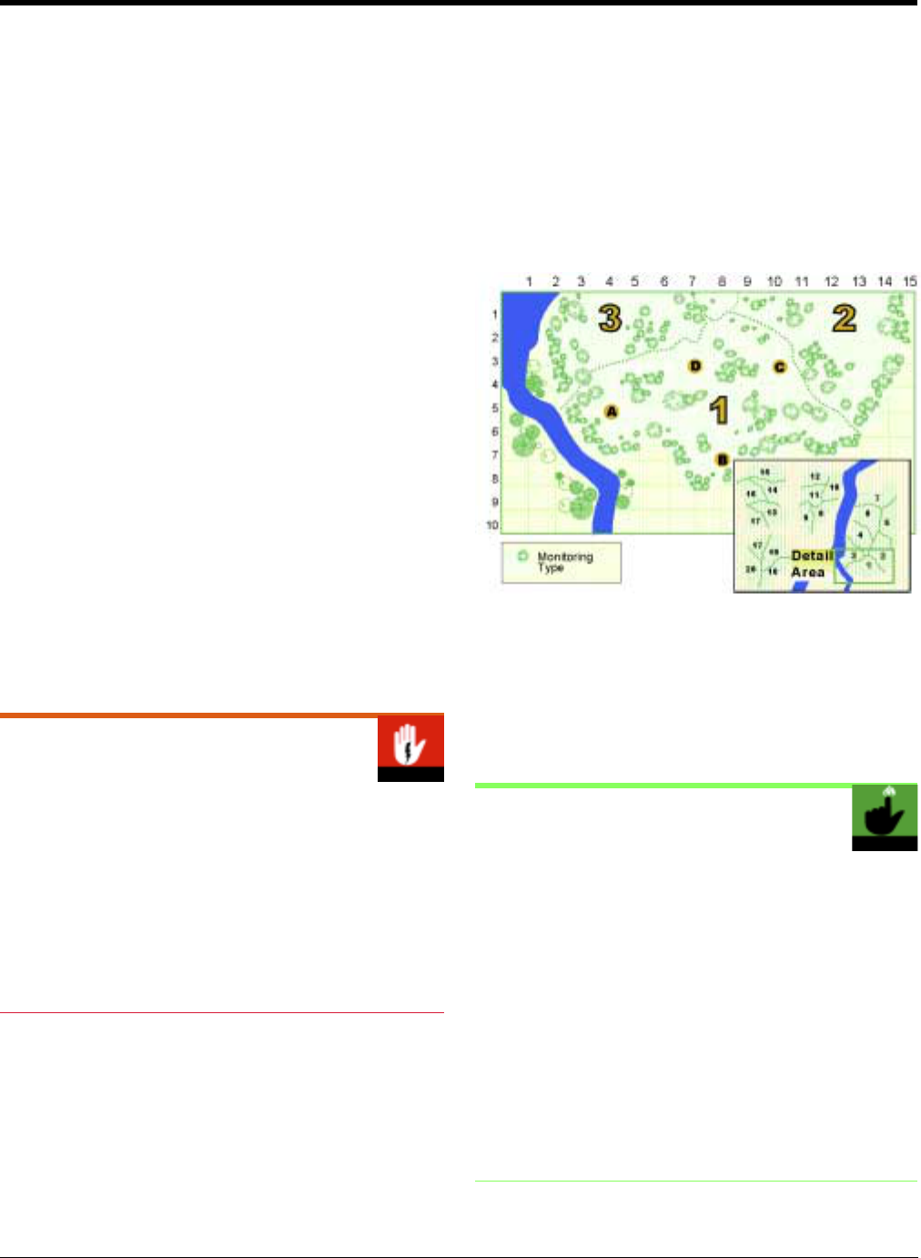
Generating Monitoring Plot Locations

First, using the restricted random sampling method

discussed below, randomly locate ten monitoring plots

per monitoring type throughout all units proposed for

prescribed burning in the next five years. These plots

will provide quantitative information for pilot sam-

pling (see page 43), and will be used to determine the

minimum sample size required to meet your monitor-

ing objectives.

To disperse your plots across the landscape, use a vari-

ant of stratified random sampling called restricted

random sampling. This randomization method

ensures that your plots are dispersed throughout your

monitoring type. First, choose the number, n, of sam-

pling units that you will need to meet your monitoring

objective. As a guideline, use an n of 10 for areas that

are small or when the variability of your objective vari-

able(s) is low. For objective variables that are moder-

ately variable, use an n of 20, and for those that are

highly variable, use an n of 30. (These numbers may be

adjusted once you have your initial 10 plots installed.)

Then divide your monitoring type into n equal por-

tions (see Figure 15). You will then choose at least

three to five (depending on the likelihood of initial plot

rejection, see below) plot location points (PLPs) per

portion. Then establish a monitoring plot within each

of these portions (see page 62).

Restricted Random Sampling

If you have currently-established plots within a moni-

toring type that were not chosen with restricted ran-

dom sampling, follow the above directions, and when

you divide your monitoring type into equal portions,

do so in such a way that each portion only has one pre-

established plot within it. You can then concentrate

your plot establishment efforts in those portions with-

out pre-established plots.

The likelihood of initial plot rejection depends on sev-

eral factors: the odds of encountering one of your

rejection criteria (e.g., large rocky areas); how your

monitoring type is distributed across the landscape

(e.g., if the type has a patchy distribution, your PLPs

may not always land in the middle of a patch); the qual-

ity of your vegetation maps (i.e., if you have poor qual-

ity maps, your PLPs may not always land within the

type); and the quality of your Monitoring type descrip-

tion sheet (FMH-4) (e.g., you may have written a more

narrow biological or physical description than you

intended, and as a result the type that you have

described only represents a small portion of the fuel-

vegetation complex that you are sampling). Most of

this information requires input from field technicians,

so initially you will need to make your best guess as to

the likelihood of plot rejection.

Figure 15. Using restricted random sampling to generate

plot locations.

In this example, the monitoring type is first divided into 20 equal

portions (notice that portion number 17 is shared between two

burn units, as the two parts of this portion combined is equal in

acreage to each of the other portions). Second, within each

portion, random points A–D (PLPs) are placed using one of the

methods described on page 60.

Locating Your First Plots

Ideally, before you burn within a new monitoring type,

you would install all your plots in that type throughout

all units proposed for burning in the next five years.

However, when fire managers have scheduled burning

to begin before you can install all your plots, a practical

alternative is to prioritize plot locations in the “n equal

portions” that fall in burn units that fire managers plan

to burn within the next year or two. To avoid biasing

your plot locations toward burn units that will burn

first, divide up your monitoring type using the afore-

mentioned guidelines for the number of “n equal por-

tions.”

Chapter 5 n

nn

n Vegetation Monitoring Protocols 59

CREATING EQUAL PORTIONS FOR INI-

TIAL PLOT INSTALLATION

Method 1: Using a Geographic Information

System

In ArcView, use the GRID function to make a 60 × 60

m grid for forest plots, and a 40 × 40 m grid for grass

and brush plots. Then, eliminate the cells in the grid

that are not in the preselected areas, i.e., the monitor-

ing type. After that, have ArcView number the gridline

intersection points from one to x. Then divide x (the

total number of points) by the number of plots you

anticipate installing, e.g., if you think you will need 25

plots, then you would divide x by 25. You can then use

the GIS method discussed on page 61, or simply use

one of the random number methods listed in Appen-

dix B, to pick your plot location points (PLPs), in

order, within each 1/25th of the monitoring type. For

a monitoring type that contains 1,000 potential plot

locations choose random numbers from 1-40, 41-80,

81-120, etc.

Method 2: Topographic Map Method

First, use a dot grid to measure the total acreage of

your monitoring type (the portion that will be burned

over the next five years). Divide the total acreage of

that monitoring type by the number of plots you antic-

ipate installing. For example, if you have 100 hectares

of monitoring type, anticipate needing 25 plots, then

divide 100 hectares by 25. Calculate how many dots on

a dot grid are needed to encompass that size portion

(the total acreage divided by the potential n equal por-

tions). Use the dot grid to then draw the boundaries of

the n equal portions (in this example, 4 hectares each)

on your map. You can then use the Grid or XY coordi-

nates methods discussed on page 61 to establish your

plot location points (PLPs).

CREATING

n EQUAL PORTIONS WHERE

PLOTS ALREADY EXIST

Method 1: Using a Geographic Information

System

Calculate the total acreage of your monitoring type,

then divide by the number of plots you plan on install-

ing. Then calculate the radius of a circle (using the

equation below) around which no other plots would be

established.

r = A ⁄ π

where:

r= radius

A = area (acreage of n equal portions)

For example, if each n equal portion equals 40 hectares,

you will need each existing plot to have a buffer of 357

m.

In this example you would use the BUFFER command

to create a 357 m buffer around each point in your

monitoring plot point coverage. This will produce 40-

hectare circles around each plot. You will then have a

polygon coverage of circles. Then use a spatial overlay

function (or CLIP command) to eliminate from your

grid all points that fall within these circles. Pull this

new coverage into ArcView and begin the GRID pro-

cess as described above.

Method 2: Topographic Map Method

Follow the directions listed in method 1 above, and

divide each portion so that each portion contains only

one previously installed plot.

RANDOMLY ASSIGNING PLOT LOCATION

POINTS

The next step is to randomly assign plot location

points (PLPs) within each of the n portions of your

monitoring type. Each of the three methods presented

here for locating a monitoring plot on a map, ortho-

photo (an aerial photograph that corresponds to a

USGS 7.5 minute quad), or other locator, presumes

that you have divided your monitoring type into n

equal portions (see above). All three methods require

very accurate base and burn unit maps before you can

begin randomization or monitoring. This step, along

with finding the equivalent field location, can actually

be the most time-consuming activity in monitoring. In

all three methods, you will need to establish a random

point, called the plot location point (PLP), from which

the plot origin point will be determined in the field.

As you use one of these three methods to select plots,

be sure to number the selected PLPs or grid units on

your map or locator—in the order that you select

them within each

n

equal portion—before going to

the field. If you can generate UTM coordinates for

Fire Monitoring Handbook 60

your PLPs, you can use these with a Global Positioning

System (GPS) unit in the field.

Discard any PLPs or grid units that meet the rejection

criteria you have identified and recorded on FMH-4,

e.g., a plot location point in a riparian area. Ideally—

with an intimate knowledge of the monitoring type

and good maps—you would identify and exclude such

areas prior to gridding and randomly selecting the PLP

or grid unit.

Method 1: Using a Geographic Information

System

You can use a Geographic Information System (GIS)

to select and record random monitoring plot origin

points in the field. In order to use GIS to randomly

assign sample plot locations you need several base car-

tographic layers. These layers should include your best

available vegetation layers as well as elevation, slope,

and aspect. It would also be useful to have a layer that

displays the location and type of all existing sample

plots.

There are currently three approaches available to ran-

domly select PLPs using GIS tools:

• ArcView extension (for version 3.1) developed by

Alaska Support Office GIS (USDI NPS 2001b)

• ArcView extension developed by SEKI GIS

• ArcInfo Grid function <Rand>

The first two approaches offer a fairly automated pro-

cedure for experienced users of ArcView. The third

approach offers the most control and flexibility for

advanced users of ArcInfo. For further information or

to obtain copies of the ArcView extensions, contact

your GIS coordinator, or visit the FMH web page

<www.nps.gov/fire/fmh/index.htm> for contacts.

Grid or XY Coordinates Method

If you use graph paper for your grid, enlarge your

monitoring type map so that each section of the graph

paper is roughly equivalent to your plot size (50 m ×

50 m for forest types or 30 m × 30 m for brush and

grassland plot types).

your monitoring type. Assign each cell of the grid a

unique number, and randomly select cells in each por-

tion (between two and ten, depending on the likeli-

hood of rejecting the plot location points; refer to

Appendix B for random number generation). The cen-

ter point of the cell is the PLP.

Method 3: XY Coordinates Method

This method is similar to the grid map method, but

uses an XY grid. Overlay an XY grid on the map or

orthophoto containing the portion of the monitoring

type. A clear plastic ruler or transparent grid works

well for this purpose. Using the lower left-hand corner

as the origin where X, Y = 0, 0, select pairs of random

numbers to define X and Y points on the grid (see

Appendix B). The intersection of the XY coordinates

on the map is the PLP. As in the grid map method, you

will randomly select a certain number of PLPs in each

portion of the monitoring type.

Method 2: Grid Map Method

The random grid map method is a low-tech method

for random selection of monitoring plots. On a map,

draw (or place) a grid atop each of the n portions of

Chapter 5 n

nn

n Vegetation Monitoring Protocols 61

Plot Location

Your randomly selected plot location points (PLPs)

(see page 60) will serve as the starting point for actual

plot location, which is done in the field. From the PLP,

you will measure a random direction and distance to a

plot origin point.

STEP 1: FIELD LOCATING PLPs

With your map of numbered PLPs in hand, you are

ready to locate plots in the field. If you generated these

PLPs using a GIS, you have UTM coordinates, and you

can use a GPS unit to find your points. To eliminate

bias, visit potential plot locations in the order in which

they were randomly selected within each portion of the

monitoring type (see page 59). This will eliminate any

tendency to avoid plots located in difficult terrain or

that are otherwise operationally less desirable.

Verify plot suitability by visiting each PLP identified on

the map. To locate your PLP, first choose a landmark

near your point that you can easily locate on your map

(or aerial photo). Determine the actual distance and

bearing from the landmark to the PLP. Once you’ve

found the landmark in the field, use a compass,

adjusted for the local declination, and measure (tape,

hip chain, or pace) the distance to the point using this

information. If your points were generated with GIS,

use of a GPS unit will greatly increase your accuracy in

locating the PLP.

Once you have found the PLP, you will select a plot

origin point. To do this, select a random compass

direction (0° to 359°) from a list of random azimuths,

which you can create using a random number genera-

tor (Appendix B).

Next, select a random distance (0 to 20 m) from a list

of random distances, which you can create using a ran-

dom number generator. Locate the plot origin point by

moving the indicated direction and distance.

Navigation Aids

If you need assistance using a compass, using declina-

tion, using a clinometer, measuring distances in the

field, or other navigation techniques, see pages 201–

206 in Appendix C.

Randomization

For each plot you plan to install, generate two or three

sets of random numbers, six random azimuths (0–359)

(one for plot location, one as the plot azimuth and four

for the fuel transects) and one random distance (0–20

m), ahead of time. An excellent idea is to generate all

the random azimuths and distances that you will need

for the entire season at once, using a spreadsheet pro-

gram (e.g., Microsoft Excel or Lotus 123) (see page

191). Make sure that you cross each number out

after you use it. In a pinch, you may generate a ran-

dom azimuth by randomly spinning the dial of your

compass. However, remember that this not the pre-

ferred method.

STEP 2: ASSESSING PLOT ACCEPTABILITY

AND MARKING PLOT ORIGIN

From the plot origin point you’ve just identified, check

the area against the monitoring type description and

rejection criteria on FMH-4 (Monitoring type descrip-

tion sheet). If the monitoring plot origin point and the

area roughly within a 50 m radius of that point meet

the criteria for the monitoring type, proceed to mark

and establish the monitoring plot.

If the origin point and surrounding area meet one or

more rejection criteria for the monitoring type, return

to the PLP, orient 180° away from the previous ran-

domly selected azimuth, and move a distance of 50 m

to a new plot origin point. If the second location meets

one or more rejection criteria, reject the PLP and pro-

ceed to the next one (return to Step 1) (see Figure 16).

Fire Monitoring Handbook 62

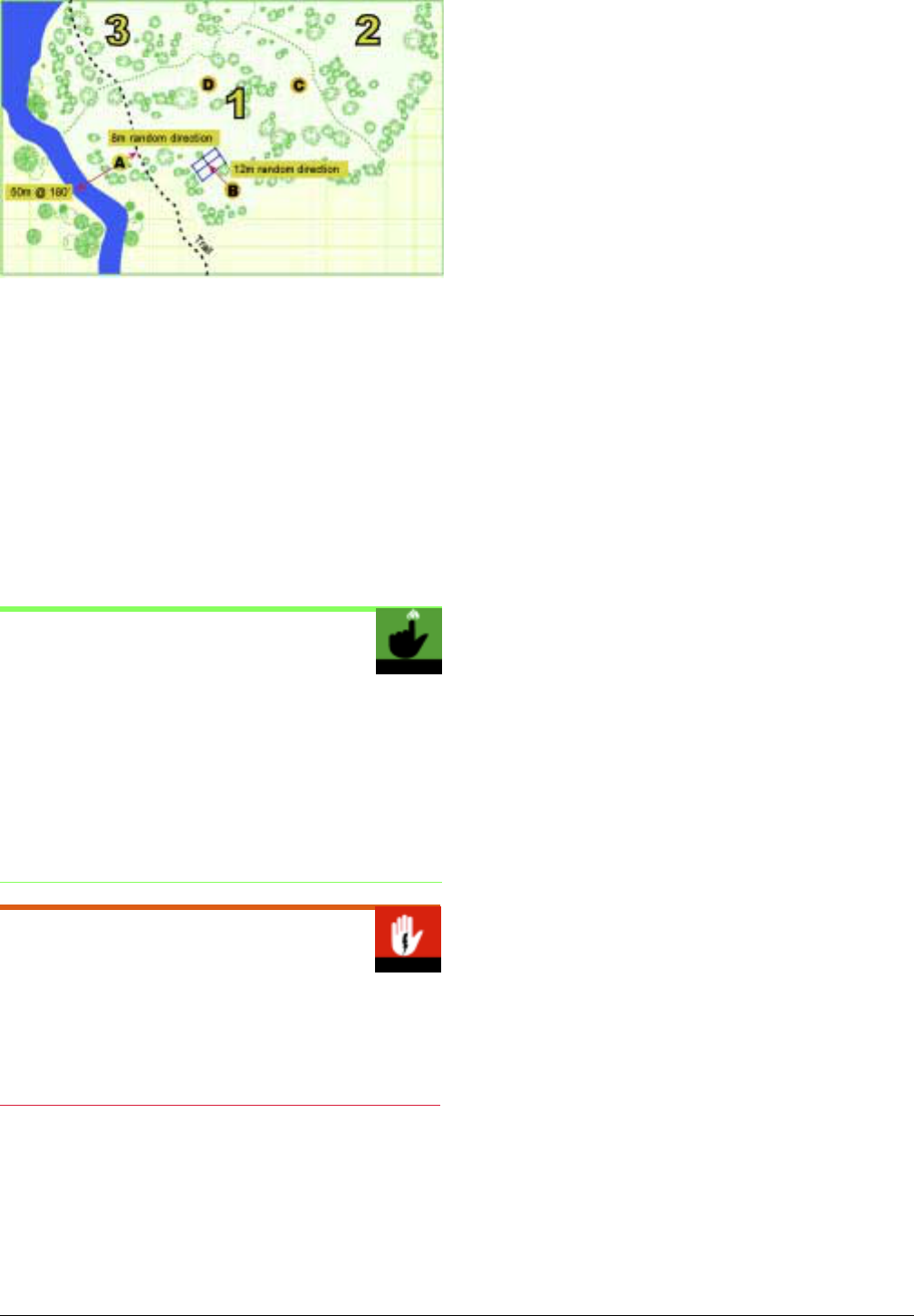
Figure 16. Initial steps of plot location.

In this example, a monitoring crew first visits PLP A and rejects

that point after trying a random number and distance, then trying

50 m at 180°. The crew successful accepted the plot near PLP B

after going a new random direction and distance from that point.

Note: PLPs were visited in the order that they were chosen (A–

D).

If the area around your origin point meets the criteria

for the monitoring type, install a stake, which serves as

the plot origin point (the center point of the forest plot

or the 0 point of a grassland or brush plot). Marking

the plot is described in detail under the plot layout and

installation section (page 64).

Increase Your Chances of

Accepting a Plot Location Point

Within narrow monitoring types (e.g., riparian, canyon

edges, and where the PLP falls at a location that would

likely lead to an acceptable plot site only within a range

of directions), the random azimuth generation may be

restricted to that range, provided that the range of

available azimuths is fairly generous (at least 60

degrees).

Working on Steep Slopes

Where steepness of the slope characterizes the moni-

toring type, wear light boots or shoes (if safe to do so)

and take extra care to minimize activity within the plot

boundaries.

Chapter 5 n

nn

n Vegetation Monitoring Protocols 63

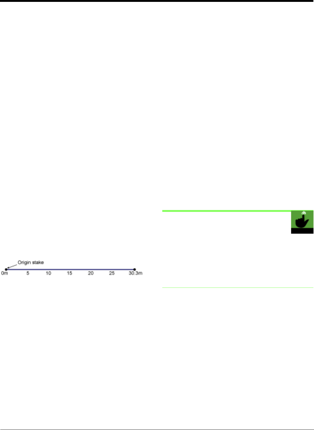
3

Laying Out And Installing Monitoring Plots

Laying Out & Installing Monitoring Plots

Plot layout and installation methods vary with plot

type; here, each method is presented separately. Two

monitors are recommended for grassland, and three

for brush plot installation. A minimum of two moni-

tors are needed for forest plot installation, but a third

and even fourth monitor will make it go more than

twice as fast and are especially important where vege-

tation is very dense. In all plots you will need your

Monitoring type description sheet (FMH-4) and Plot

location data sheet (FMH-5), a compass, and stakes.

Stake labels (tags) are used in all types of plots and are

discussed following the section on forest plot layout

and installation. For a complete equipment list, see

Appendix E.

GRASSLAND AND BRUSH PLOTS

As described earlier in this chapter (page 62) you have

generated a plot origin point from your PLP, and have

marked this point by installing an origin stake. From

this origin stake, select a random azimuth (Appendix

B) and lay out a 30 m+ tape from the origin stake

along this azimuth (see Figure 17). Suspend the

transect line, defined by the tape, above the vegetation

(brush plots may require special techniques—see tip

on page 65). This may require construction of two tri-

pod scaffolds—one for each end of the tape. The

entire 30 m line and 5 m on either side of it must lie

within the identified monitoring type.

Figure 17. Grassland or brush monitoring transect.

Place a stake at each point marked with a black circle (•). Note

that the endpoint is installed 0.3 m past the endpoint of the

transect to minimize interference.

Mark the Plot

Mark the transect dimensions by installing two 0.5 in

diameter rebar (rebar is recommended throughout the

text, but other materials may be used, see Appendix E)

stakes at 0 and 30.3 m. Installing a stake at 30.3 m

(30P) minimizes stake interference in the point inter-

cept transect at the 30 m data point. Stake height

above the ground should allow easy relocation of the

stakes. Stakes should be installed deep enough to pro-

vide adequate basal stability relative to the height nec-

essary to bring the stake into view. Suggested stake

lengths are 0.5 to 1 m for grassland transects, and 2 m

or more for brush transects. It is generally best to

overestimate the stake heights needed, to compensate

for snow creep and vegetation growth.

Burial of the origin stake (0 point) is recommended,

especially in areas subject to vandalism or disturbance.

A metal detector (or magnetic locator) can be used

later to relocate the plot if all of the above-ground

stakes are lost. In high-use areas it may be necessary to

partially camouflage stakes, or to mark beginning and

end points with buried metal markers that can be relo-

cated with a metal detector (or a magnetic locator).

Electronic Marker Systems, or “cyberstakes,” may be

useful under these circumstances (see page 224).

Color code plot beginning and ending stakes (orange

for 0P, blue for the 30P) with heat-resistant paints, e.g.,

automotive engine paint. Place a piece of cardboard

behind the stake while you are painting it to protect the

surrounding vegetation. Repaint the stakes after each

burn.

Install permanent plot identification tags on each stake

as described on page 70.

Defining the Brush Belt

You may find it useful to define the brush belt for

future monitors by installing two additional stakes,

each a belt width away from 0P and 30P. These two

stakes should be 30 m apart instead of the 30.3 m dis-

tance separating 0P and 30P.

Fire Monitoring Handbook 64

Advice for Installing Brush Plots

Shrubland types can be very difficult (and sometimes painful) to navigate in, make straight lines through and pho-

tograph. Here are some tips to aid intrepid shrubland monitors.

• The best way to string a straight tape in a shrubland depends on the height, density and pliability of the species

concerned. If the average height of the shrubs is <1.5 m, pound the rebar to within a decimeter or two of the

average height (use rebar long enough for you to bury a third to half of the stake), and string the tape over the

top of the vegetation. If the shrubs are >1.5 m and have a relatively open understory, run the tape along the

ground. However, if these tall shrubs are fairly continuous, you may be better off trying to string the tape right

through the stems. No matter how you string the tape, record on the FMH-5 where you string it, so future

monitors can replicate your work.

• Three may be the best number of monitors for installing brush plots, with two people setting up the transect

and the third mapping and photographing. When re-reading the plot, two people can collect transect data and

the third can collect density data and photograph the plot.

• When on slopes, approach the plot from above. You will find it easier to move, toss equipment, and sight from

above than below. Examine where your plot might go, and plan out your sampling strategy to minimize move-

ment from one end of the plot to the other.

• Play leapfrog to navigate to the plot, or when stringing the tape along the azimuth. The first person sights along

the azimuth while the second person moves through the brush to the farthest point at which she or he can still

see the first person. Note: Rather than trampling directly down the actual transect line, take a circuitous route.

Two monitors will sight on each other trading the compass and the tape. Then the first person works his or her

way around past the second person to the next point where a line of sight can still be maintained. They sight on

each other once again and toss the tape, and continue until the destination is reached.

• Use a tall, collapsible, brightly painted sampling rod and include it in your photos. This will make the opposite

stake (0 or 30P) more visible in the photos, and will let your fellow monitors know where you are.

• Wear a brightly colored shirt, hat or vest. Flag the sampling rod. Flag your glasses. Flag your hat. Do whatever

you have to do to be seen.

• In addition to using a GPS unit to record the plot location, make the plot easier to find by installing reference

stakes or tagging reference trees, and locating at least three other highly visible reference features. Take bearings

to three of these features, so that returning monitors can locate the plot by triangulation.

• You may find it useful to set up a photo point from an adjacent ridge to get a community-wide view of change

over time.

Chapter 5 n

nn

n Vegetation Monitoring Protocols 65

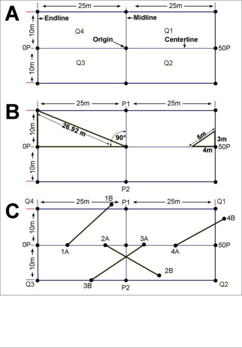
Figure 18. Steps in laying out a forest plot.

A) place stakes at points marked with a black circle (•); B) lay out 90° angles and adjust the corner stakes; C) place remaining plot

stakes.

Fire Monitoring Handbook 66

FOREST PLOTS

Locate the Plot Origin

For forest plots, your origin point (see page 62),

marked by a stake, serves as your plot center (see

Figure 18A).

Establish the Plot Centerline

You will use this origin to lay out a rectangular

plot (Figure 18). Select a random azimuth (Appendix

B) and measure a 50 m line along this azimuth, using

the origin point as its center. The centerline is defined

by a tape measure laid as straight as possible. To lay out

this 50 m tape, stand at the plot origin and run the 0

end of the tape toward the 0P point (along the back

azimuth) and the 50 m end of the tape to the 50P

(Figure 18A). Record the plot azimuth on the Forest

plot data sheet (FMH-7).

Establish the Plot Boundaries

Laying out the tape to define the plot boundaries

requires at least two monitors—one for each end. The

monitors must take time to lay out the plot as a true

rectangle. These plots are large and one monitor could

lose sight of the other, making it difficult to “square”

the plot corners (90° angles). A few helpful hints to

accomplish this task are provided here.

Lay out the plot centerline as straight as possible. Next,

lay out three 20 m (or 30 m) tapes perpendicular to the

centerline, also as straight as possible, and such that

the tapes intersect at right angles. Start with either line

P1–P2 or Q4–Q3. To accomplish this use the principle

of the 3, 4, 5 triangle. For every right angle, measure 3

m along the 20 m tape where it intersects the center-

line; mark the measurement. Measure 4 m along the

centerline; mark the measurement. The hypote-

nuse of the resulting triangle should be 5 m (as illus-

trated in Figure 18B). If the hypotenuse is not 5 m,

adjust the 20 m tape so that it is.

In sparsely vegetated forest types you may be able

to triangulate using larger triangles. For example,

in Figure 18B the hypotenuse of the triangle from the

centerline 0P to point P1 is 26.92 m.

Lay out the endline (Figure 18A) and midline tapes,

making sure that the “0" end of each tape starts at the

same end of the plot.

If the plot encompasses variable slopes, such as a

ravine (and this does not cause you to reject it), lay out

the tapes so that you are measuring slope distance (see

Glossary) rather than horizontal distance—FMH.EXE

software will correct for this. In such a case, it will be

impossible to perfectly square the plot, but this allows

for the most true representation of the area on the

ground. For plots with a understory of dense shrubs,

see page 65 for tips on installing plots in brush.

Plot Squaring Priorities

Squaring a plot can be tedious and time-consuming.

Keep in mind that the variables affected by this pro-

cess are density of overstory, pole-size and possibly

seedling trees. The degree to which the plot should be

perfectly square depends on the density of trees, partic-

ularly if there are any trees right on the boundary in

question. If trees are dense and there are one or more

trees on the boundary, it is important to get the cor-

ners as square as possible. A good guideline is that the

3, 4, 5 triangle be no more than 1 dm off on each side.

If trees are sparse and there are no trees on the bound-

ary, squareness is less critical and an error of 30 dm

may be acceptable. Accuracy Standards: ± 0.5 m

for the length, and ± 0.2 m for the width, of a for-

est plot (Table 8, page 69).

Orient the Plot Quarters

Once your plot is squared, divide the plot into quarters

and assign numbers according to the following proto-

col. If you stand at the plot origin, with both feet on

the centerline and the 0 point (0P) on your left, Quar-

ter 1 (Q1) is to your forward-right. Quarters 2, 3,

and 4 are numbered clockwise from Q1 as shown

in Figure 18A.

Carrying Rebar

If you backpack into your plots, try using the bottom

of a plastic soda bottle to carry your rebar stakes, in

order to protect your pack.

Mark the Plot

Define the plot, quarters, and fuel inventory lines as

shown in Figure 18C with rebar stakes (rebar is recom-

mended throughout the text, but other materials may

be used, see Appendix E). Bury a 0.5 in diameter rebar

stake (the origin stake) at the plot center or origin.

Install rebar stakes at each of the four corners of the

20 m × 50 m plot (Q1, Q2, Q3, and Q4) and at the

starting points along the centerline for the four fuel

Chapter 5 n

nn

n Vegetation Monitoring Protocols 67

inventory transects (1A, 2A, 3A, and 4A). Place a stake

at either end of the center line (points 0P and 50P),

and a stake at either end of the short axis midline

(points P1 and P2).

Define the end points of the fuels inventory lines by

installing rebar stakes at these points (1B, 2B, 3B, and

4B) using four random azimuths. Often the end points

of the fuel transects will be 50 ft from the beginning

points (A), but in some types they may be longer.

Check the protocols (FMH-4) and install to the appro-

priate length.

Stake height above the ground should be sufficient to

allow easy relocation of the stakes. Install the stakes

deep enough to provide adequate basal stability relative

to the height necessary to bring the stake into view.

Suggested stake lengths are: 0.5 m–1 m for forest

plots, or taller if undergrowth is tall and thick. It is gen-

erally best to overestimate the stake heights needed, to

compensate for snow creep and vegetation growth.

Burial of the plot reference or origin (center) stake is

recommended, especially in areas subject to vandalism

or disturbance. The other key stakes (Q1, Q2, Q3, Q4,

0P, and 50P) may also be considered for burial, but

only as a last choice, as buried stakes can be difficult to

install, locate, and remove. Buried stakes can be relo-

cated with a metal detector (or a magnetic locator).

Color-code the plot beginning and ending stakes

(orange for 0P, blue for the 50P) using heat-resistant

paints, e.g., automotive engine paint. Repaint the stakes

after each burn.

Park managers will have to determine whether plot

marking standards recommended in this handbook are

appropriate for their unit. This handbook calls for the

placement of seventeen 0.5 in diameter rebar stakes for

each forest plot. These markers are important for the

relocation of plots and transects. In some situations,

however, these rebar stakes may be hazardous,

destructive to cultural resources, or visually or philo-

sophically intrusive. Plastic caps placed on the top of

the stakes may prevent injuries and can increase stake

visibility (and in some places are required by law). At

an absolute minimum, the origin stake and the four

corner stakes (Q1, Q2, Q3, and Q4) must be installed.

These stakes can be camouflaged by paint or by total

or partial burial. You may also consider using “cyber-

stakes” (see page 224). Any innovations or deviations

from the above should be well documented.

Plots are distinguishable from one another through

identification codes etched onto metal tags which

attach to the rebar stakes. Directions for preparing and

installing these tags follow this section.

Large Obstructions Encountered on

the Transect

Follow this procedure if you encounter a large obstruc-

tion, like a very large tree or tall rock, along a forest

plot boundary line (refer to Figure 19):

• Lay the tape straight, along the transect, until the

point at which the obstruction is encountered.

• Pound a permanent stake at this point.

• Deviate from the transect at a 90-degree angle in the

direction enabling the shortest offset, until you are

clear of the obstruction, and pound a temporary

stake there.

• Lay the tape to the end of the obstruction, following

the original transect azimuth, and pound another

temporary stake there.

• Measure and record the distance between the two

temporary stakes.

• Divert 90 degrees again back to where the original

line would pick up and pound another permanent

stake.

• At this point, you may remove the temporary stakes

and secure the tape back at the permanent stake

preceding the obstruction.

• Add the distance measured between the two tempo-

rary stakes to the distance on the tape at the point at

which the deviation was made and the first perma-

nent rebar was installed.

• Unwind a second tape out to this distance and

attach it at this point to the permanent stake follow-

ing the obstruction, then lay the remainder of it out

to the end of the transect.

• If this occurs on a transect on which herbaceous

and woody plant data are collected, the code for the

obstruction (2BOLE, 2RB, etc., see Table 15,

page 86) is recorded for each missed interval.

Fire Monitoring Handbook 68

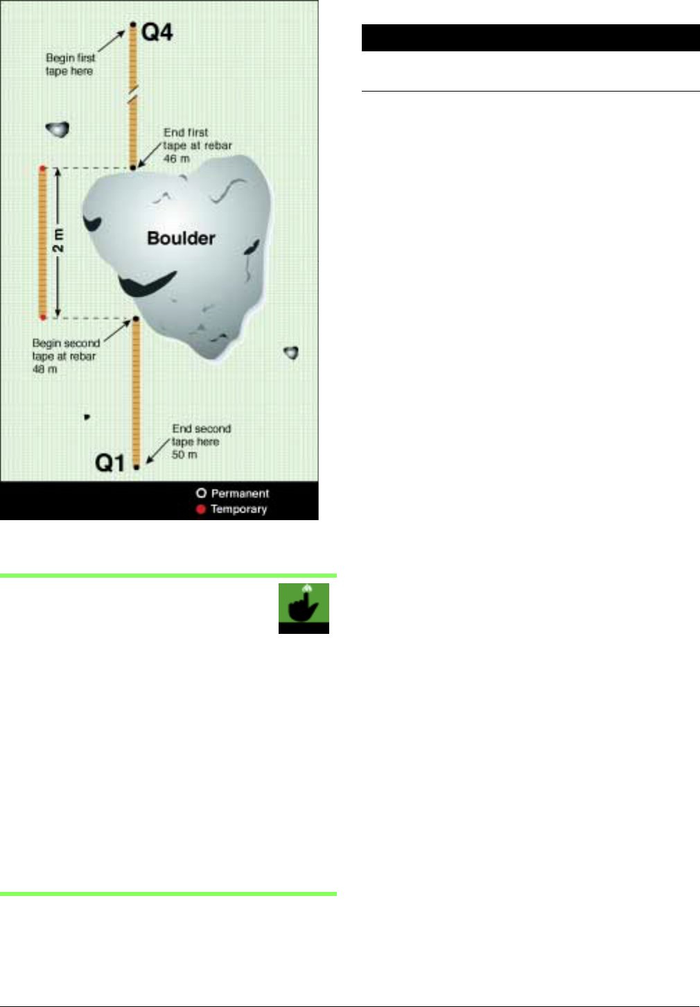
Table 8. Accuracy standards for plot layout.

Plot Layout

Dimensions ± 0.5 m (or 1%), forest plot length

± 0.2 m (or 1%), forest plot width

Figure 19. Procedure for circumventing a large transect

obstruction.

When The Rebar Won’t Go In

At times rebar cannot be satisfactorily pounded into

the ground. If this is the case at one of your plot

points, try installing the rebar out a little further along

the tape, or sinking it in at an angle so that the top is

in the correct location. You can also use a “rock drill”

or cordless drill to drill holes prior to placing rebar (in

areas that are subject to seasonal flooding, it may be a

good idea to secure them with marine epoxy). Alter-

natively, you can pile up rocks around the rebar, but

only if that won’t affect the variable you are sampling

and the cairn has a reasonable chance of remaining

undisturbed.

Chapter 5 n

nn

n Vegetation Monitoring Protocols 69

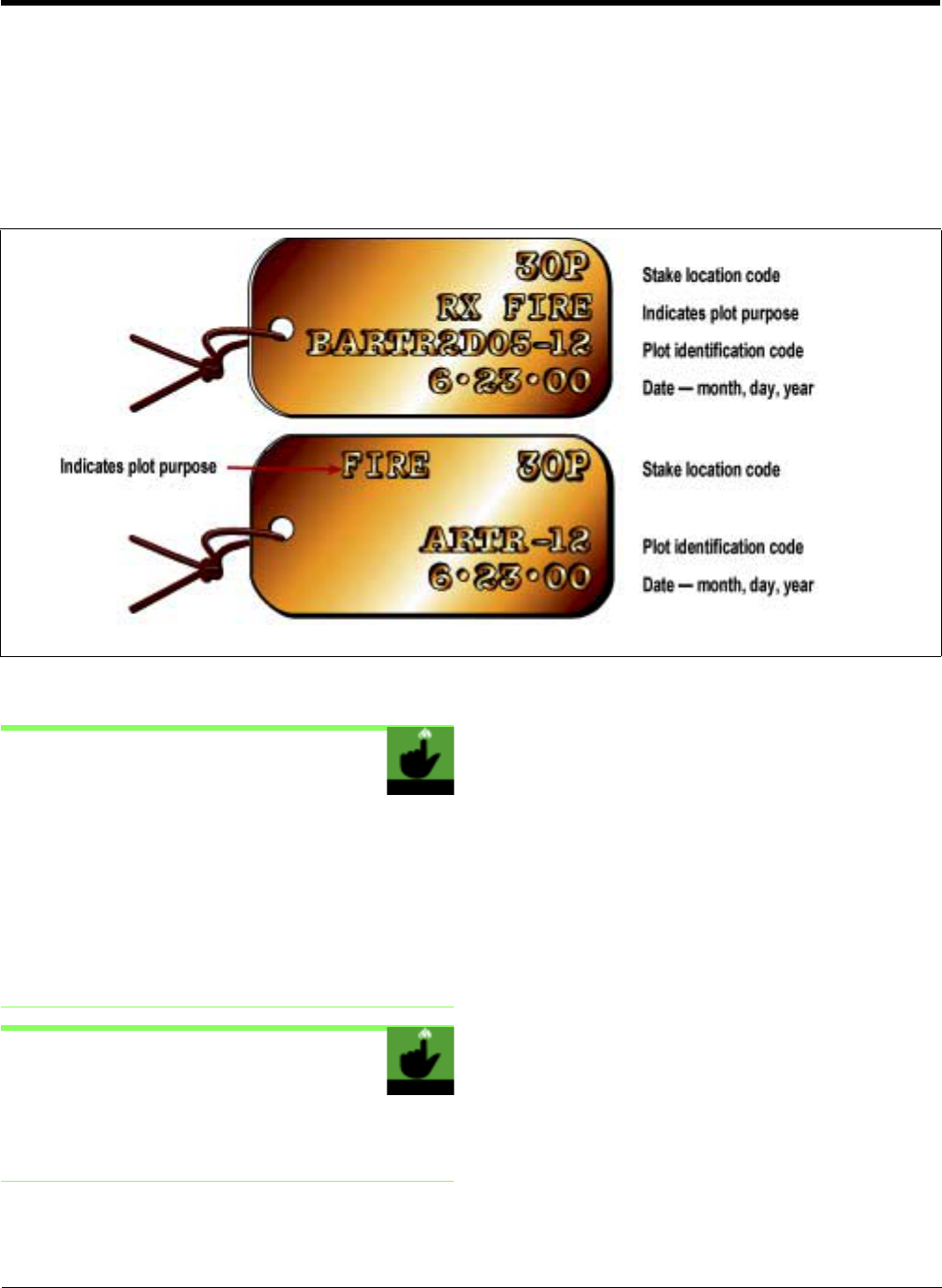
3

Labeling Monitoring Plot Stakes

Install permanent plot identification tags on each stake

as described below.

• Use rectangular or oblong brass tags; aluminum

tags are likely to melt (Appendix E).

• Each tag should include the monitoring stake

location code, plot purpose, plot identification

code, and date of initial installation. An abbrevi-

ated format may be used to reduce the amount of

minting. It includes the monitoring stake location

code, plot purpose, vegetation code from the plot

identification code, plot number and date. The

two formats are displayed in Figure 20.

Figure 20. Two formats for labeling plot stake tags.

The stake location codes are identified in Figure 17, page 64 (brush or grassland plots) and Figure 18, page 66 (forest plots).

Save Time Stamping

Stamping the tags using a die set produces the most

wear-resistant results, but is very time-consuming.

Stamp the tags (except the date and the plot number,

which can be added once the plot has been accepted)

before going into the field and consider stamping only

the Q1, Q2, Q3 Q4 and Origin stake tags, and using an

electric engraver to encode the others in the field.

Nonstandard Stamp Additions

You may find it useful to include the plot azimuth or

other additional information on each tag.

Fire Monitoring Handbook 70

Photographing the Plot

Once all the tapes are laid out, take a minimum of two

photos at each grassland or brush plot (Table 9), and

eight photos at each forest plot (Table 10), following

the “Subject” sequence listed below (also included on

FMH-7). If necessary to better characterize the vegeta-

GRASSLAND AND BRUSH PLOTS

Table 9. Sequence for grassland and brush plot photos.

tion at the site, take additional photos from a well-doc-

umented location. To minimize the effect of

vegetation trampling on the photo, photograph the

monitoring plot before you sample other variables,

staying outside the plot as much as possible.

Subject Code

1. From 0P toward 30P 0P–30P

2. From 30P toward 0P 30P–0P

3. From 0P toward reference feature 0P–REF

4. From reference feature toward 0P REF–0P

FOREST PLOTS

Table 10. Sequence for forest plot photos.

Subject Code

1. From 0P toward the Origin stake (plot center) 0P-Origin

2. From stake Q4 toward stake Q1 Q4-Q1

3. From stake P1 toward the Origin stake P1-Origin

4. From stake Q1 toward stake Q4 Q1-Q4

5. From 50P toward the Origin stake 50P-Origin

6. From stake Q2 toward stake Q3 Q2-Q3

7. From stake P2 toward the Origin stake P2-Origin

8. From stake Q3 toward stake Q2 Q3-Q2

9. From the Origin toward reference feature Origin–REF

10. From reference feature toward Origin REF–Origin

RS PROCEDURES

• A coded photograph identification “card” (see

photo card tip below) should be prepared and

made visible in every photograph. The card

should display, in large black letters, the plot iden-

tification code, date (if camera is not equipped

with a databack), subject code and any other infor-

mation that may be useful, e.g., park code, burn

unit, or burn status.

• Use the same kind of camera, lens, and film

each time you rephotograph. Note: Use rela-

tively stable technology such as 35 mm cameras

and film rather than the latest digital camera. Try

to retake the photo at the same time of day, and at

about the same phenological stage of the shrub

and herbaceous species. To avoid shadows, take

photographs when the sun is directly overhead,

when possible.

• Place a flagged rangepole or other tall marker at

the midpoint or the end of the line being photo-

graphed. The pole should be located at the same

point each time the plot is rephotographed. This

can provide for clearer comparisons over time.

Chapter 5 n

nn

n Vegetation Monitoring Protocols 71

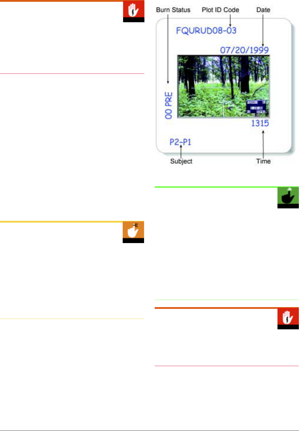
Photographic Protocols

The following procedure differs from that recom-

mended in previous versions of this handbook. Previ-

ously established photopoints should always be

rephotographed using the protocols that were used

when the points were originally established.

• Using a tripod or monopod, raise the camera to a

height of 4 ft and set it back from the starting point

just far enough to get the top of the closest stake in

the field of view. Exactly how you frame the shot

will also depend on the slope and horizon—on a

hillside or ravine, angle the camera with the slope.

Align the camera horizontally for the recommended

photos. Take an additional vertical shot, if that bet-

ter characterizes the plot, due to an obstruction,

dense shrubs, tree bole, large rock, etc., in the cam-

era’s field of view. Make sure that the light meter

reading doesn’t include any sky. If it does, first point

the camera at the vegetation only and note the read-

ing given there, then reposition the camera. The

photo should include the tape as well as the stakes

at either end of the transect along which you are

shooting.

Rephotographing Plots

Remember that when you are photographing plots that

have already burned, you should make every attempt

to duplicate the preburn photos, no matter what tech-

nique was used, unless the previous photos are poor,

e.g., pictures of plot stakes, but not the plot itself. If

possible, bring a reference photo (a color photocopy

of the original) along to facilitate duplication of earlier

shots.

• Basic photography guidelines can be found on

page 207 in Appendix C.

• Record photographic information on the Photo-

graphic record sheet (FMH-23 in Appendix A).

• As soon as the film has been developed, label all

slides as per Figure 21. The Photographic record

sheet should be used as a reference. It may be

helpful to add the park code if more than one park

is served by the same monitoring team.

Figure 21. Suggested format for labeling slides.

Importance of Good Preburn Photos

The importance of the highest quality preburn data

cannot be overemphasized. Returning to plots to

retake photos is costly and time-consuming, but abso-

lutely necessary if you take poor photos the first time.

This is especially critical at the preburn stage as the

value of postburn photos is dependent upon good pre-

burn photos for comparison. Extra time and care

taken to get good photos the first time will be repaid,

as poor quality images will require a return visit to the

plot to reshoot the photos.

Taking Slides into the Field

Never take original slides into the field; they will be

degraded by light exposure and abrasion, and could be

lost entirely.

EQUIPMENT AND FILM

Use a 35 mm camera with a 35 mm lens. A 28 mm lens

will give you an even wider field of view, but may be

harder to come by. A databack camera may be used to

ensure that the date and time are recorded on the film,

but is not necessary. In the near future, high resolution

Fire Monitoring Handbook 72

digital cameras may become the best technology for

photo documentation. However, as of this writing, the

quality of camera necessary to produce clear, well-

defined projectable slides is prohibitively expensive for

most monitoring programs. Note: Choose one type of

equipment and use it for the duration of the monitor-

ing program.

Use the highest quality film type available for long-

term storage. Exposure to UV light is extremely detri-

mental to image longevity, and light damage is cumula-

tive. At this writing, the most stable slide film available

for long-term dark storage is Kodachrome, however it

is unstable when exposed to light, especially projector

bulbs. Fujichrome has superior projection-fading sta-

bility. A balance should be sought between projector-

fading and dark fading stability (Wilhelm and Brower

1993). Under the best storage conditions, slides from

both films will last up to fifty years. Note: Some pro-

grams may want to consider using black and white

prints for archival purposes. This medium will hold up

longer than slides, and allows for very nice visual com-

parisons, but can be costly and require a lot of storage

space for programs with an extensive plot network.

Choose film speed according to the amount of light

generally available in the monitoring type, or likely to

be available during the data collection visit. At times

this could necessitate changing the film mid-roll and

rewinding it for later use or wasting the remaining film

on the roll, but this is preferable to poor photo quality

and will be less expensive than having to return to the

plot to rephotograph it if the photos are not accept-

able. More details on film and basic photography

guidelines can be found starting on page 207.

Chapter 5 n

nn

n Vegetation Monitoring Protocols 73

Successful Photos

• Always bring a copy of the preburn photos into the field to facilitate replication of earlier shots. This can be a

set of photographic prints, scanned images, color photocopies or slide duplicates generated for this purpose

and included in the “field packet” (see page 112).

• Photos will be more useful if they show primarily the vegetation, and space taken up by the board and moni-

tor is minimized. Have someone hold the board so that the codes are just visible in each photograph, but the

board itself is as unobtrusive as possible. While it would make for great reminiscing, the person holding the

board and the other data collectors should not be visible in the photo.

• A convenient photo board can be fashioned out of a piece of white paper (or card stock) laminated with 10

mil plastic; dry erase markers can then be used to mark the board. Such a board will last one field season. For

a more permanent tool, try using a dry erase board, or a magnetic board as developed by the Glacier National

Park sign shop (details are provided in Appendix E).

• Use the same lens focal length each time you rephotograph.

• If it is not clear what the best camera settings are, bracketing the photos (taking three photos of the same sub-

ject using a range of settings) will decrease the chance that a revisit will be necessary.

• If the closest stake that should be in the photo is obstructed by a shrub or tree limbs, take the photo anyway,

flagging the stake and moving as little vegetation as possible. You may then take an oblique shot of the photo

transect if desired, noting the exact location from which this shot was taken and that this photo should always

be repeated on subsequent visits.

If obtrusive vegetation prevents you from placing the camera in such a spot that you can get the closest stake

in the picture, it may be acceptable to take the photo while standing at the stake itself, or from a different

height (but not above 5 ft), as long as this is noted and repeated on all subsequent visits, even if the intruding

vegetation is later consumed. Never prune vegetation from a plot.

• Retake the photo when the shrub and herbaceous species are at the same phenological stage as they were in

the original photos.

• Processing slides promptly will allow you time to retake poor photos while the vegetation is still at the pheno-

logically correct stage.

• If you find that the Photographic record sheet (FMH-23) is too large, or if you use multiple cameras, keep a

small notebook with appropriately labeled pages in the camera bag at all times. Attaching the notebook to the

camera bag will reduce the risk of losing the entire notebook and all the data with it.

Fire Monitoring Handbook 74

Field Mapping the Monitoring Plot

Copies of your field maps should be included in each

plot folder, in the “field packet,” and possibly also in a

general monitoring type file (see page 112 for a discus-

sion on field packets and plot folders). Note the loca-

tion of monitoring plots on each of the following types

of maps:

• USGS 7.5-minute or 15-minute topographic quad,

detailed trail map, GIS map, or best available map

for your park

• Orthophoto quad or aerial photo, if appropriate

(note that in open country, aerial photos can make

relocation of the monitoring plots much easier,

but they are not as useful in closed forest types)

• Hand-drawn route map, including a plot diagram

and reference features

• Full park or small-scale map (for inclusion in a

monitoring type or monitoring program general

file)

Mapping

Those who follow in your footsteps won’t have your

footsteps to follow. When mapping, keep in mind that

your map may be used by monitors who are unfamiliar

with your park, and make the map as clear as you pos-

sibly can. Include as many geographic features as pos-

sible to reassure future monitors that they are on the

right course, and indicate when they have arrived.

Remember to include enough information (e.g., azi-

muths and distances to multiple reference features) in

your maps for future monitors to easily recreate the

plot if one or more rebar are missing. This is especially

critical for grassland and brush plots, as they have only

two stakes. Note: Accuracy standards for plot location

measurements are located in Table 11, page 76.

Reference Features

In difficult terrain, or for distances longer than your

longest tape, use a Global Positioning System (GPS)

unit to find the azimuth and distance from the refer-

ence feature to the plot. For assistance using a GPS

unit, see page 205 in Appendix C.

COMPLETE PLOT LOCATION DATA SHEET

Follow along with the completed Plot location data

sheet (FMH-5) on page 77 as you read the steps on the

following two pages. A blank FMH-5 is available in

Appendix A.

• Assign and record the plot identification code.

The plot ID number consists of the monitoring

type code (see page 36), and a two digit plot num-

ber; ex.: FSEGI2T08–01 or BARTR2D05–01. The

last two digits (plot number) should start with 01

for each monitoring type and continue sequen-

tially within each type.

• Circle whether the plot is a burn plot or a control

plot (B/C). Record the date you completed the

form, the burn unit name or number (or both),

the people that completed the form, the topo-

graphic quad containing the plot, the azimuth of

the transect, and the declination (see page 202)

that you used for all azimuths.

• Record Universal Transverse Mercator values

(UTMs) or longitude and latitude. If appropriate,

record township and range as well. Record

whether the location was determined with a map

and compass or a GPS unit. If you use a GPS unit,

record the Position Dilution of Precision (PDOP)

or Estimated Horizontal Error, 2D (EHE) if you

are using a PLGR, and specify the datum used

(e.g., North American Datum-1927, NAD27). See

page 205, Appendix C for a discussion of PLGR

use and datums. Note: If you map the location of

the plot with a GPS unit on a date different from

that on which you installed the plot, be sure to

note this on the History of site visits (FMH-5A).

• Record the average percent slope that the plot azi-

muth follows, the average percent slope, the

aspect, and elevation (from a GPS unit or a topo-

graphic quad) of the plot location.

• Describe the fire history of the plot. At a mini-

mum, include the date of the last fire, if known.

• Record the travel route used to access the moni-

toring plot (also show this on a topographic map).

• Record the true compass bearing (includes decli-

nation) followed from the road or trail (or other

relatively permanent reference point) to locate the

monitoring plot. Mark on the topographic map

Chapter 5 n

nn

n Vegetation Monitoring Protocols 75

where you left this well-known trail or road, and

photograph this location if necessary.

• Describe how to get to the monitoring plot, refer-

ring to the hand-drawn map. Note: Some people

can easily follow written directions, while others

prefer visual directions. Use the hand-drawn map

to illustrate the written directions by including all

your geographic references, including the highly

visible features from which you took bearings.

• Identify permanent or semi-permanent reference

features on the site in case the origin stake is hard

to find or disappears. The reference feature

should be easy to relocate, such as an obtrusive

and distinctive living tree or large boulder, peak,

or cliff. Install a reference stake if no reference

features are available, but use them sparingly and

place them carefully to avoid attracting vandalism.

• Record the true compass bearing (includes decli-

nation) and distance in meters from the reference

feature to the origin stake.

• Describe the plot location accurately and thor-

oughly, referring to the hand-drawn map.

• Complete the History of site visits (FMH-5A)

every time you visit the plot.

• Enter the FMH-5 into the FMH database

(Sydoriak 2001).

• Fill out the Forest plot data sheet (FMH-7); see

the warning box below.

Forest Plot Data Sheet (FMH-7)

The Forest plot data sheet (FMH-7) has been modified

from a photo record sheet to a place where you can

record the azimuth and slope of each fuel transect line

and draw in the transect lines and the sampling areas

for overstory, pole and seedling trees. See the example

on page 79.

Table 11. Accuracy standards for plot location description.

Plot Mapping

% Slope ± 5%

Elevation ± 100 ft (30 m)

UTM ± 30 m (by GPS unit)

± 100 m (by hand)

Lat/Long ± 2 seconds (by GPS unit)

± 5 seconds (by hand)

Fire Monitoring Handbook 76

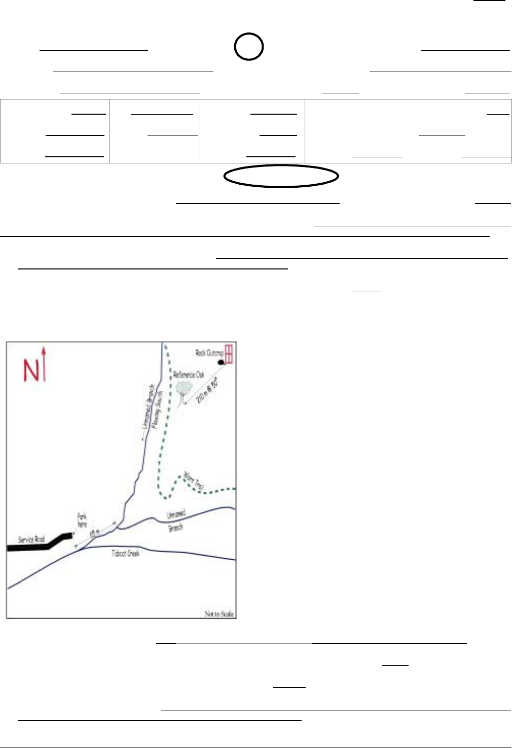
Park/Unit 4-Character Alpha Code:

GRSM

FMH-5 PLOT LOCATION DATA SHEET

Plot ID:

FPIRIG08–04

B / C (Circle One) Date:

7 / 31/ 00

Burn Unit:

RCW

Recorder(s):

Blozan, Feeley

Topo Quad:

Calderwood

Transect Azimuth:

134°

Declination:

3°W

UTM ZONE:

UTMN:

UTME:

Lat:

35° 32'30"

Long:

85°55'0"

Section:

Township:

Range:

Slope (%) along Transect Azimuth:

10%

Slope (%) of Hillside:

23%

Aspect:

224°

Elevation:

1360'

Location Information Determined by (Circle One): Map & Compass / GPS

If determined by GPS: Datum used: (Circle One) PDOP/EHE:

Fire History of the Plot (including the date of the last known fire):

Burned in a wildland fire (human caused

ignition) in 1971 and (natural ignition) in 1958. Additional information is unavailable prior to 1943.

1. Road and trail used to travel to the plot:

Take 441 from park headquarters to 321; make a left on

321. Take 321 to Route 129; turn left on Route 129.

2. True compass bearing at point where road/trail is left to hike to plot:

50

°

3. Describe the route to the plot; include or attach a hand-drawn map illustrating these directions,

including the plot layout, plot reference stake and other significant features. In addition, attach a

topo, orthophoto, and/or trail map.

Plot can be reached from Route 129 beginning at the

utility line service gate. Follow the service road

under the power lines and over the crest of small,

steep hill toward Tabcat Creek. Continue following

the road upstream (southeast). The road will cross

the stream three times, the third being a relatively

wide and shallow section (2.1 mi. to third crossing).

This crossing is also a split in the service road. Veer

left and continue up Tabcat Creek, following the

overgrown service road, crossing first under the four

strand power lines and then the main lines (twin

sets). You may have to cross the stream several

times for ease of passage. Travel upstream to the

junction of an unnamed creek branch, 0.6 mi from

service road split and 250 m east of Cattail Branch

on the north side of Tabcat. The road becomes

impassible at this point, park here. Follow the branch

65 m (paced) to its junction with a tributary flowing

almost due south. A worn trail will be apparent east

of the creek. Cross the creek and follow the trail up

to the crest of the ridge and look for a lone, stately

old chestnut oak (Quercus prinus, DBH 83 cm) with a

tag on its south side. The tag says: RXFire

FPIRIG08 Ref.#1. From the tagged oak, travel 210

m (paced) at 50° to Q3. The plot is located on the

northeast side of a large rock outcrop.

4. Describe reference feature:

Q. prinus, DBH = 82.8 cm

5. True compass bearing from plot reference feature to plot reference stake:

50

°

6. Distance from reference feature to reference stake:

210

m

7. Problems, comments, notes:

It is difficult to see the plot until you are almost upon it. The Q4–Q1

line goes to the uphill side of the large boulder at 39 m.

Chapter 5 n

nn

n Vegetation Monitoring Protocols 77

FMH-5A HISTORY OF SITE VISITS

Plot ID:

FPIRIG08–04

B / C (Circle One) Burn Unit:

RCW

Date

Burn

Status

Purpose Comments

7/28/00 PRE Install Plot/Begin Data Collection

7/31/00 PRE Complete Data Collection

9/8/00 01 Burn Burn Plot, Collect Fire Behavior data Only ½ of the Plot Burned

10/22/00 01 Post Replace Tag 2A,OT Tags 29–32

6/17/01 01 yr01 Data Collection Identified 2GRAM3!

7/13/01 01 yr01 Retake 01 Yr01 Photos 6/17 Photos Too Dark

5/11/02 01 yr02 Data Collection GPS Plot Location

5/4/05 01 yr05 Data Collection 2B Stake Is Missing

5/20/05 01 yr05 Replace 2B Stake

6/23/10 01 yr10 Data Collection

8/24/10 02 Burn Burn Plot, Collect Fire Behavior data Entire Plot Burned

10/5/10 02 Post Data Collection Q3 & 0P Rebar Missing

2/2/11 Reinstall Rebar

6/17/11 02 yr01 Data Collection

Fire Monitoring Handbook 78

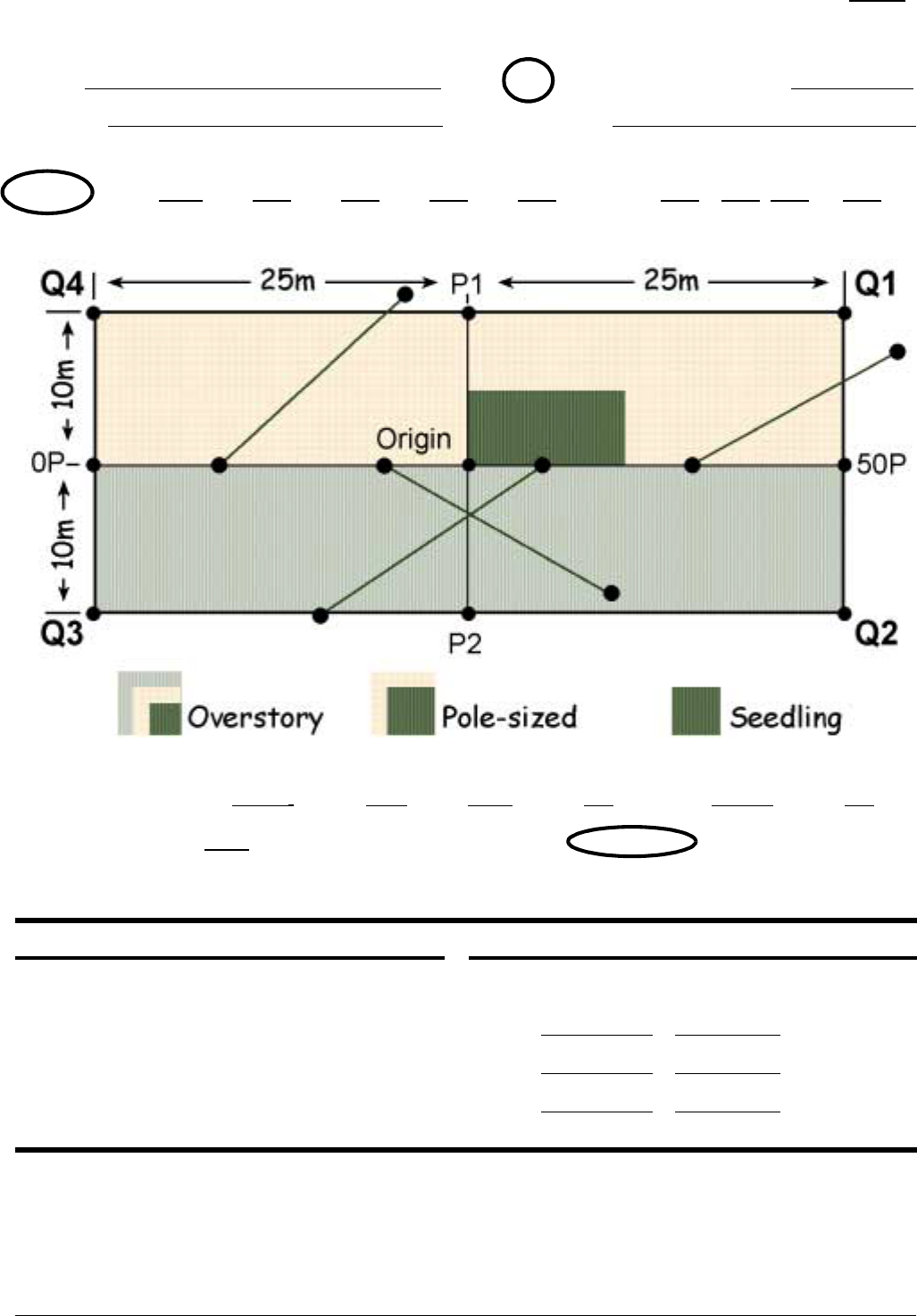
Park/Unit 4-Character Alpha Code:

GRSM

FMH-7 FOREST PLOT DATA SHEET

Plot ID:

FPIRIG08–04

B / C (Circle One) Date:

7 / 31 / 00

Burn Unit:

RCW

Recorders:

Blozan, Feeley

Burn Status:Circle one and indicate number of times treated, e.g., 01-yr01, 02-yr01

00-PRE POST -yr01 -yr02 -yr05 -yr10 -yr20Other: -yr ; -mo

Overstory:

1,000

m

2

in Q

1–4

Pole:

250

m

2

in Q

1

Seedling:

62.5

m

2

in Q

1

Sampling

Shrub:

150

m

2

along Q4–Q1 w Q3–Q2 w 0P–50P Q4–30 mw

Areas:

Shade in the sampling areas for each tree class and for the shrub sampling area(s) on the

plot layout above.

Photo Subject Order Fuel Load Transects

1. 0P

Ł Origin 6. Q2 Ł Q3

Azimuth Slope

2. Q4

Ł Q1 7. P2 Ł Origin

1

234° 3%

3. P1 Ł Origin 8. Q3 Ł Q2 2

130° 12%

4. Q1 Ł Q4 9. Origin Ł REF 3

41° 5%

5. 50P Ł Origin 10. REF Ł Origin

4

323° 7%

Record photo documentation data for each visit Draw in fuel load transect lines on the plot layout

on FMH-23, Photographic record sheet above.

Chapter 5 n

nn

n Vegetation Monitoring Protocols 79

Monitoring Vegetation Characteristics

ALL PLOT TYPES

This section describes specific methods for data col-

lection. Each variable may be sampled in various levels

of intensity depending on the monitoring type charac-

teristics. These protocols are predetermined for each

monitoring type; sample each variable the same way

for every plot within a monitoring type (see page 43).

Before you begin data collection, refer to the Monitor-

ing type description sheet (FMH-4) and review the

exact protocols to be followed for each specific moni-

toring type. For quick reference, use the Forest plot

data sheet (FMH-7) to record and shade in the sam-

pling areas for overstory, pole-size and seedling trees;

see previous page.

Accuracy Standards

Accuracy standards for each variable are listed at the

end of each subsection of this chapter.

Form Headings

Fill out the form heading completely. Record the mon-

itoring plot ID code, whether it is a burn plot (B) or a

control plot (C), the date the data were collected, the

burn unit name or number, the names of the data col-

lector and recorder (in that order), and the burn status

(with the first two digits referring to the treatment

number, and the last four letters and numbers referring

to the visit relative to the last treatment). For example,

01 yr02 refers to a year-2 data collection visit the next

sampling season after the first burn or other treatment

(thinning, etc.), 03 Post refers to the immediate post-

burn data collection following the third burn or other

treatment. Preburn data are always coded 00 PRE, but

if preburn data are updated before the first burn, the

code for the original preburn data in the database will

change to 00 PR01. If preburn data are collected a

third time before the plot burns, the second preburn

data will be re-coded 00 PR02 and so on. The code 00

PRE is always used for the newest set of preburn data.

Streamlining the Form Filling

Process

Fill out form headings (minus the date and recorders)

and other transferable information (fuel transect azi-

muths, tree tag numbers, etc.) before you go into the

field. Forms can be assembled for each plot during

slow periods in the office, during bad weather, or when

there is a little extra time.

Before You Visit a

Previously Established Plot

Use the Plot maintenance log (FMH-25) to document

any items that you notice during a plot visit that need

to be attended to during the next plot visit. Once you

establish a plot, maintain the plot log and update it

after each visit. By reviewing this log before visiting the

plot, you can gather the necessary items to “fix” the

problem noted previously. This form provides a reli-

able method of communication with monitors of the

future. Examples of plot maintenance needs: replace-

ment of a tag that was missing on the last visit, a miss-

ing rebar, or verification of a species identification.

HERBACEOUS AND SHRUB LAYERS

RS Procedures

Use form FMH-16 for 30 m transects or FMH-15 for

50 m transects (both are found in Appendix A). Use a

point intercept method to record the number of

transect hits and to obtain relative and percent cover

by species over time. On forest and brush plots, also

measure shrub density within a brush belt for the same

distance, along the same transect. The collection of

voucher specimens is strongly recommended; this is

discussed on page 87.

Fire Monitoring Handbook 80

Be Kind to the Fragile Herbage, Fine

Fuels and Soils Beneath Your Feet

In order to minimize the effect of trampling on the

data, stay outside the plot as much as possible, and

sample forest types in the following sequence:

• Lay out tapes

• Photograph plot

• Collect herbaceous and shrub data, and fuels data

(decide which layer is the most fragile, and collect

those data first)

• Collect seedling tree data

• Collect overstory and pole-size tree data

Avoid heavy boots in favor of light shoes; set down

sampling equipment, backpacks etc., to the side or

below the plot, not in or above it; and minimize the

number of people working in the plot. Additionally,

use extreme caution on steep slopes.

Herbaceous and Shrub Layer Accu-

racy Standards

Accuracy standards for each variable discussed in this

section are listed at the end of this section (Table 16,

page 90).

Locate the 0 point on the point intercept transect

The data collection starting point is at the 0P (origin

stake) on grassland and brush plots, and the Q4 (and

possibly Q3 and 0P) on forest plots. The length and

number of transects is determined during the monitor-

ing design process (Chapter 4). Check your protocols

on the Monitoring type description sheet (FMH-4)

before proceeding.

Collect number of transect hits—grassland, brush

and forest types

Start 30 cm from the 0P or Q4. Drop a ¼ in diameter

pole (a rigid plumb bob), graduated in decimeters, gen-

tly so that the sampling rod is plumb to the ground (on

slopes this will not be perpendicular to the ground),

every 30 cm along the transect line. Where the transect

length is 30 m, there will be 100 points from 30 to

3,000 cm. On forest plots where the transect is read

along the full 50 m, there will be 166 points from 30 to

5,000 cm. In either case, the first intercept hit is at 30

cm, not at 0.

At each “point intercept” (Pnt), gently drop the pole to

the ground, and record each species (Spp) that touches

the pole on the appropriate data sheet (FMH-16 for

grassland and brush plots, FMH-15 for most forest

plots, and FMH-16 for forest monitoring types that

use only the Q4–30 m line). Count each species only

once at each point intercept even if the pole touches it

more than once. Record the species from tallest to the

shortest. If the pole fails to intercept any vegetation,

record the substrate (bare soil, rock, forest litter, etc.

(see Table 15, page 86)). Note: You can occasionally

find vegetation under a substrate type; in this case you

would ignore the substrate and record the vegetation.

If the rod encounters multiple types of substrate,

record only that which the pole hits first.

Do not count foliage or branches intercepted for trees

over 2 m tall, but count all other vegetation, including

shrubs, no matter its height. (This is because trees are

better sampled using other procedures, and the target

variables using the point intercept transect are shrubs

and herbs.) If the sampling rod intersects the bole of a

tree that is over 2 m tall, record “2BOLE,” or

“2SDED” if the tree is dead. Note: Record species not

intercepted but seen in the vicinity (in a belt on either

side of the brush and herbaceous layer transect) on the

bottom of the data sheet (FMH-15 or -16). The width

of this belt is specified on your Monitoring type

description sheet (FMH-4).

Note: If you have selected to use the point intercept

method to calculate basal cover (see page 46), record

only the bottom hit for each point, regardless of

whether it is substrate or vegetation.

Sampling Rods

A useful sampling rod can be made in any of sev-

eral ways. Choose one that best suits your needs

(see Table 12, page 82). One-dm markings can be

made with an engraver, then filled in with a permanent

marker; road paint and road sign adhesives can also be

useful. Note that surface marking with most pens or

paints wears off quickly, and many adhesives get gooey

in the heat.

Chapter 5 n

nn

n Vegetation Monitoring Protocols 81

Table 12. Types of sampling rods.

Pole Type Pros Cons

Fiberglass Rod: Moderately available None to note.

This is the pre- (your maintenance shop

ferred choice. may already have

some, or you can buy a

bicycle whip (remove

the flag)), moderate in

price, lightweight, easy

to carry, can be screwed

together to adjust size

and all pieces need not

be carried if not needed,

very durable.

Tent Pole: Fiber- Readily available (sport- Possibly hard

glass with shock ing good store), moder- to find 0.25”

cord. This is the ately priced, lightweight, diameter,

second choice. foldable, durable. shock cord can

break.

Steel Rod: Readily available (hard- Bend, heavy,

ware stores), moder- difficult to carry

ately priced, extremely in the field.

durable.

Wooden Dowel: Readily available (hard- Fragile, incon-

ware stores), cheap, venient to

lightweight. carry.

Tall Vegetation

Sampling Problems

If your protocols (FMH-4) require you to record

height and the vegetation is unexpectedly taller than

the sampling rod, try dropping the rod at the sampling

point, then placing your hand at the 1 or 1.5 m point

on the rod and sliding the rod up (without looking up),

elevating it by 1 or 1.5 m and recording where it

touches the vegetation above you. If the vegetation is

consistently taller, find a taller sampling rod.

Dead Herbaceous and Shrub Species

Sampling Problems

You may encounter dead standing vegetation along

your transects. Always record dead annual vegetation

in the same way you record live individuals. Record

dead biennial and perennial vegetation (except dead

branches of living plants) by placing a “D” at the end

of the species code. This permits dead vegetation to be

treated separately from live vegetation. Dead perenni-

als may not be included in species abundance indices,

but their presence may provide information for esti-

mating fire behavior and determining mortality. In gen-

eral (see the warning box below for exceptions) count

dead branches of living plants as a live intercept. In

the case of shrub and herbaceous species, this also

applies if the main plant is dead but sprouting, and the

dead part is encountered.

Counting Dead Branches of Living

Plants as Dead (Optional)

In some cases, such as where animal habitat or aerial

fuels are a concern, you may want to know the cover of

dead branches, regardless of whether they are attached

to living bases. If your monitoring type requires it, you

may count dead branches of living plants as dead.

However consistency is essential—if transects were

not initially read this way for a monitoring type, a

change “midstream” will cause an apparent dip in the

cover of live shrubs that is not necessarily true.

Sprouting Dead Trees

Trees under 2 m tall: If the bole (>2 m tall) is dead

but sprouting at the base, consider any live sprout (<2

m tall) you encounter as live.

Trees over 2 m tall: If you encounter a live basal

sprout over 2 m tall, the sprout should be considered a

tree (2BOLE) in its own right.

Fire Monitoring Handbook 82

Optional Monitoring Procedures

Shrub and herbaceous layer height

At every sampling point, measure the height of the tall-

est living or dead individual of each species (to the

nearest decimeter, in meters) at the highest place on

the sampling rod touched by vegetation. Record this

height (Hgt) on FMH-15 or -16. A ¼ in wide sampling

rod graduated in decimeters should make this mea-

surement relatively easy. Do not record data for aerial

substrate such as the leaves or stems attached to a dead

and downed tree.

Record Species Codes

Species codes are assigned in a systematic way follow-

ing Natural Resource Conservation Service methodol-

ogy, as used in the USDA PLANTS Database (USDA

NRCS 2001). For existing programs, see the warning

box below. This naming convention uses a 4–7 charac-

ter alpha code beginning with the first two letters of

the genus name and the first two letters of the species

name. The following 0–3 characters are assigned as

needed to avoid confusion of plants with duplicate

codes. If there is no subspecies or variety, the next

character(s) may not be needed or will simply be a one

or two digit number representing the alphabetical

ranking of that plant on the national list.

Examples:

DACA Dalea californica

DACA3 Danthonia californica

DACA13 Dasistoma calycosa

If the plant is a subspecies or variety, then the charac-

ter in the fifth position will be the first letter of that

infraspecific name, and if there are duplicates, a num-

ber will follow.

Examples:

ACRUT Acer rubrum var. trilobum

ACRUT3 Acer rubrum var. tridens

DACAP Dalea carthagenensis var. portoricana

DACAP3 Danthonia californica var. palousensis

Assigning Species Codes

If you have an existing monitoring program it is not

necessary to look up every species in your Species code

list (FMH-6). The FMH.EXE software will convert

your species codes for you.

If you are starting a new program, simply enter the

genus, species, and infraspecific name (if appropriate)

into the FMH.EXE software, and the software will

look up the species code for you.

When you add a new species to the database, you must

note certain other information as well. This includes

the species code, its lifeform (see the warning box

below) the full name, whether the species is native or

non-native, and whether it is annual, biennial, or

perennial. This information is recorded on the Species

code list (FMH-6).

Life Form

Life form categories and their codes are as follows; see

Glossary for full definitions.

A - Fern or fern ally S - Shrub

F - Forb T - Tree

G - Grass U - Subshrub

N - Non-vascular V - Vine

R - Grass-like * - Substrate

Blank - Unknown, non-plant

Note: If blank is selected, you may also leave the fol-

lowing codes blank—whether the species is native or

non-native, and whether it is annual, biennial, or peren-

nial.

The FMH-6 serves as a running list of species codes.

Keep only one list for the entire monitoring program

in a given park, to avoid assigning incorrect codes. You

should carry this sheet whenever you are collecting

data, and you should refer to it every time you assign a

species code. If you are unsure of the official code for

a new plant (see page 83 for coding guidelines), assign

a temporary code, then correct it on your data sheets

and species list once you look up the official code.

Once you enter the initial data into the FMH software

(Sydoriak 2001), you may print out the Species code

list from the database. Using this form will keep the

Chapter 5 n

nn

n Vegetation Monitoring Protocols 83

same code from being used for two different species,

and will greatly facilitate data processing.

Dealing with unknown plants

Use an identification guide to make every attempt to

identify every plant to the species (and subspecies or

variety) level. If you cannot identify a plant because

you need to have specific parts (e.g., flowers, fruits,

etc.) not available during your sampling time (see

page 199 for guidance on identifying dead and dor-

mant plants), or you need to use a dissecting scope,

take steps to allow future identification. Collect the

plant (from off the plot), label it, describe it in

detail, and then press it (see page 193 for guidelines on

voucher collections). Assign an unknown code that is

unique from all other unknown codes in the park and

note a detailed description of the plant.

ALWAYS collect (or draw) and describe unknowns in

the field, so that future field technicians will record the

same unknown with the same code.

Management of unknown species can easily get out of

hand, especially if there is a turnover of monitors from

year to year, the flora is particularly diverse and com-

plex, monitors are overworked or monitors lack the

requisite plant identification skills. The remedies for

these conditions are obvious: try to retain monitors

from year to year, stress good documentation and

quality, hire monitors who are trained in plant identifi-

cation, and be realistic about their workload. But even

under the best of circumstances, you will encounter

the occasional unknown species.

Here are some tips that may help you keep your

unknowns straight and get them identified.

• Keep meticulous notes including a detailed,

botanical description of all the plant parts, loca-

tion and micro-habitat, as well as any guesses as to

genus or species.

Example:

Plants are herbaceous, 15–25 cm tall (but have been

browsed) with several stems originating from the

base. Leaves are 2–3 cm long, 0.5–1 cm wide, alter-

nate, oblanceolate with finely dentate margins, gla-

brous above and tomentose below. Leaf tips are

acuminate. No fruits or flowers are present. Plant is

occasional in light openings in the ponderosa pine

understory.

• Collect the plants (off the plot) and sketch if nec-

essary.

• Make vouchers for the herbarium, but be sure to

also make a set of field reference vouchers for

unknowns.

• Refer to the vouchers or field reference often

throughout the season to see if last year’s

unknown is this year’s well-known friend.

• Keep a list of unknowns with notes as to why they

were not able to be identified. Review the list in

the early season and make a special trip to try to

get the plants that were encountered after they

had flowered and fruited.

• Scout around in similar areas for other individuals

that may be more easily identifiable.

• Ask an expert, in park or out. Botanically-minded

folk from a nearby university or the local native

plant club are usually more than happy to help.

Also consider taking digital photos and distribut-

ing them over the Internet to groups who have

botanical expertise.

Assign each unknown plant a unique code; make every

effort to match up duplicates of the same unknown.

The PLANTS database has a series of default codes

for unknowns (Table 13), and genera (see database

(USDA NRCS 2001)). If you have more than one

unknown (whether vascular or non-vascular) that

matches the code of the category or where you can

only key it to genus, then add a number to the codes as

shown below. Note: Some genera have numbers at the

end of their codes; always check the PLANTS database

to be sure that the code you intend to use is not used

by another genus or species. In the example below, the

code for Dryopteris is DRYOP, however the code

DRYOP2 is used for Dryopetalon, so monitors had to

use numbers starting with 3 to avoid conflicts.

Fire Monitoring Handbook 84

Examples:

2GLP1 for unknown perennial grass number

1 (a densely tufted grass, with basal

and cauline flat spreading leaves, hairy

ligules)

2GLP2 for unknown perennial grass number

2 (a loose rhizomatous grass, with

rolled basal and cauline leaves, no

ligules)

DRYOP3 for unknown Dryopteris number 1 (pet-

ioles less than one quarter the length

of the leaf, blade elliptic, 2-pinnate,

marginal teeth curved, growing on

limestone)

DRYOP4 for unknown Dryopteris number 2 (pet-

ioles one-third the length of the leaf,

scales with a dark brown stripe; blade

deltate-ovate, 3-pinnate, pinnule mar-

gins serrate)

Table 13. Species codes for unknown vascular plants.

2FA

2FB

2FD

2FDA

2FDB

2FDP

2FERN

2FM

2FMA

2FMB

2FMP

2FORB

2FP

2FS

2FSA

2FSB

2FSP

2GA

2GB

2GL

2GLA

Forb, annual

Forb, biennial

Forb, dicot

Forb, dicot, annual

Forb, dicot, biennial

Forb, dicot, perennial

Fern or Fern Ally

Forb, monocot

Forb, monocot, annual

Forb, monocot, biennial

Forb, monocot, perennial

Forb (herbaceous, not grass nor grasslike)

Forb, perennial

Forb, succulent

Forb, succulent, annual

Forb, succulent, biennial

Forb, succulent, perennial

Grass, annual

Grass, biennial

Grasslike (not a true grass)

Grasslike, annual

Table 13. Species codes for unknown vascular plants. (Ctd.)

2GLB

2GLP

2GP

2GRAM

2GW

2PLANT

2SB

2SD

2SDB

2SDBD

2SDBM

2SDN

2SE

2SEB

2SEBD

2SEBM

2SEN

2SHRUB

2SN

2SSB

2SSD

2SSDB

2SSDBD

2SSDBM

2SSDN

2SSE

2SSEB

2SSEBD

2SSEBM

2SSEN

2SSN

2SUBS

2TB

2TD

2TDB

2TDBD

2TDBM

Grasslike, biennial

Grasslike, perennial

Grass, perennial

Graminoid (grass or grasslike)

Grass, woody (bamboo, etc.)

Plant

Shrub, broadleaf

Shrub, deciduous

Shrub, deciduous, broadleaf

Shrub, deciduous, broadleaf, dicot

Shrub, deciduous, broadleaf, monocot

Shrub, deciduous, needleleaf

Shrub, evergreen

Shrub, evergreen, broadleaf

Shrub, evergreen, broadleaf, dicot

Shrub, evergreen, broadleaf, monocot

Shrub, evergreen, needleleaf

Shrub (>.5m)

Shrub, needleleaf (coniferous)

Subshrub, broadleaf

Subshrub, deciduous

Subshrub, deciduous, broadleaf

Subshrub, deciduous, broadleaf, dicot

Subshrub, deciduous, broadleaf, monocot

Subshrub, deciduous, needleleaf

Subshrub, evergreen

Subshrub, evergreen, broadleaf

Subshrub, evergreen, broadleaf, dicot

Subshrub, evergreen, broadleaf, monocot

Subshrub, evergreen, needleleaf

Subshrub, needleleaf (coniferous)

Subshrub (<.5m)

Tree, broadleaf

Tree, deciduous

Tree, deciduous, broadleaf

Tree, deciduous, broadleaf, dicot

Tree, deciduous, broadleaf, monocot

Chapter 5 n

nn

n Vegetation Monitoring Protocols 85

Table 13. Species codes for unknown vascular plants. (Ctd.)

2TDN

2TE

2TEB

2TEBD

2TEBM

2TEN

2TN

2TREE

2VH

2VHA

2VHD

2VHDA

2VHDP

2VHM

2VHMA

2VHMP

2VHP

2VHS

2VHSA

2VHSP

2VW

2VWD

2VWDD

2VWDM

2VWE

2VWED

2VWEM

Tree, deciduous, needleleaf

Tree, evergreen

Tree, evergreen, broadleaf

Tree, evergreen, broadleaf, dicot

Tree, evergreen, broadleaf, monocot

Tree, evergreen, needleleaf

Tree, needleleaf (coniferous)

Tree

Vine, herbaceous

Vine, herbaceous, annual

Vine, herbaceous, dicot

Vine, herbaceous, dicot, annual

Vine, herbaceous, dicot, perennial

Vine, herbaceous, monocot

Vine, herbaceous, monocot, annual

Vine, herbaceous, monocot, perennial

Vine, herbaceous, perennial

Vine, herbaceous, succulent

Vine, herbaceous, succulent, annual

Vine, herbaceous, succulent, perennial

Vine, woody

Vine, woody, deciduous

Vine, woody, deciduous, dicot

Vine, woody, deciduous, monocot

Vine, woody, evergreen

Vine, woody, evergreen, dicot

Vine, woody, evergreen, monocot

Make frequent checks of new unknowns against exist-

ing unknowns throughout the field season to avoid

assigning the same code to two different species, or

two different codes to the same species. Become famil-

iar with your unknowns so that you can be on the

lookout for the plant in a stage that is more easily iden-

tifiable. If the unknown is identified at a later date, the

code (ex.: 2VWE1, etc.) must be corrected globally

throughout your data sheets and in the FMH database.

The FMH software will automatically change a species

code in all databases when you change it on the FMH-

6 data form.

Non-vascular plants

For the plants that you may have difficulty identifying,

e.g., non-vascular plants like bryophytes, fungi, and

algae, you can use broad codes as shown below.

Table 14. Species codes for non-vascular plants.

2AB

2AG

2ALGA

2AR

2BRY

2CYAN

2FF

2FJ

2FR

2FSMUT

2FUNGI

2HORN

2LC

2LF

2LICHN

2LU

2LW

2MOSS

2PERI

2SLIME

Alga, Brown

Alga, Green

Alga

Alga, Red

Bryophyte (moss, liverwort, hornwort)

Cyanobacteria, cryptobiotic/cryptogamic/microbi-

otic/microphytic soil or crust

Fungus, fleshy (mushroom)

Fungus, Jelly

Fungus, Rust

Fungus, Smut

Fungus

Hornwort

Lichen, crustose

Lichen, foliose

Lichen

Lichen, fruticose

Liverwort

Moss

Periphyton

Slime Mold

Dead or inorganic material

Dead or inorganic material should be coded in the fol-

lowing way (Table 15):

Table 15. Codes for dead or inorganic material.

2BARE

2DF

2LTR

2LTRH

2LTRL

Bare ground, gravel, soil, ash; soil particles <1 in

diameter.

Forest duff. Duff is the fermentation and humus

layer. It usually lies below the litter and above

mineral soil.

Vegetation litter. Forest litter includes freshly

fallen dead plant parts other than wood, including

cones, bracts, seeds, bark, needles, and

detached leaves that are less than 50% buried in

the duff layer.

Litter, herbaceous

Litter, lichen

Fire Monitoring Handbook 86

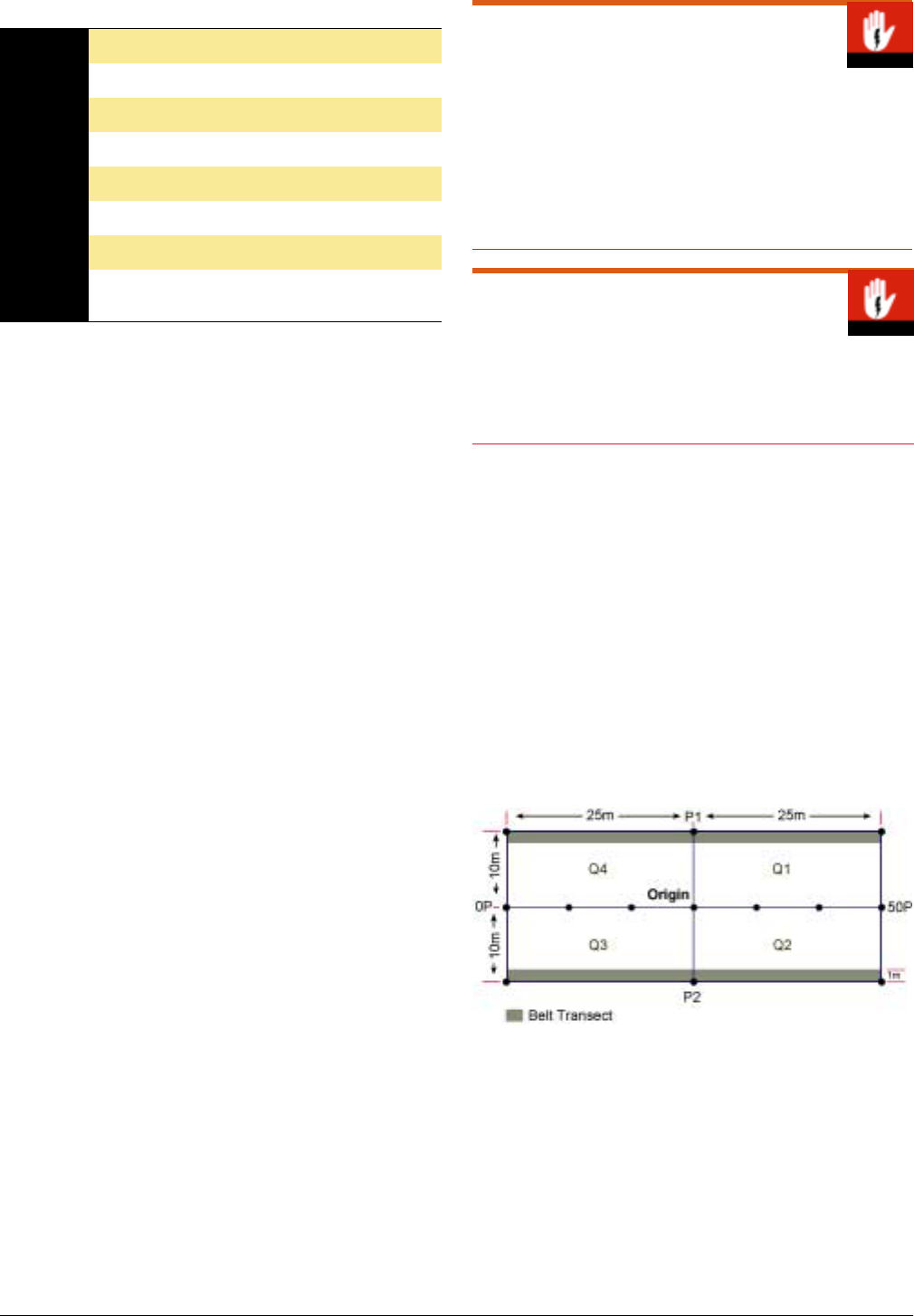
Table 15. Codes for dead or inorganic material. (Ctd.)

2LTRWL

2LTRWS

2RB

2RF

2SC

2SDED

2ST

2W

Litter, woody, >2.5 cm

Litter, woody, <2.5 cm

Rock, bedrock or mineral particles >1 in diameter.

Rock, fragments <1 in diameter.

Native, exotic, and feral animal scat.

Standing dead tree.

Tree stump, no litter at intercept point.

Water; permanent body of water or running water

present six months of the year or more.

Make Voucher Collection

General protocols for collecting voucher specimens

are included here; a detailed discussion on collecting,

processing, labeling and preserving plant specimens is

located in Appendix C. Collect vouchers when there is

any doubt as to the identification of a plant species

recorded in the data set, unless the species is threat-

ened or endangered, or the plant cannot be found out-

side of the plot.

Identify specimens within two days. Prompt identifica-

tion is essential for data accuracy, and saves time and

money. For the initial phase of this monitoring pro-

gram, collection of voucher specimens of all plants

present is strongly recommended.

Collection of vouchers using the following guidelines

(which are the same for all plot types) should enable

consistent and correct identifications:

• Collect the voucher specimen off or outside of the

monitoring plot. Collect enough of the plant to

enable identification. Do not collect plants that

are—or are suspected to be—rare, threatened, or

endangered; sketch these plants and take pictures

as vouchers.

• Press the plant materials immediately, but retain

some unpressed flowers for easier identification.

• Record collection information on a form (see

page 195) that you press with the voucher speci-

men.

• Keep all specimens in proper herbarium storage.

See Appendix C for more information on proper

herbarium storage.

• A field notebook of pressed specimens (including

unknowns) is a very useful way to verify species

identifications in the field.

Documenting Rare Plants

Do not collect a plant that is or may be rare,

threatened, or endangered! Sketch or photograph

these plants and substitute pictures for vouchers. In all

cases your collection should follow the one in twenty

rule: remove no more than one plant per twenty plants;

remove no plants if there are less than twenty.

Voucher Label

The handbook now contains a voucher collection data

sheet. You will find this data sheet on the back of the

Species code list (FMH-6).

BRUSH AND FOREST PLOTS

Collect and Record Shrub Density Data

Record shrub density along a brush belt adjacent to

the point intercept transect. The width of this belt is

specified on your Monitoring type description sheet

(FMH-4). Count each individual having >50% of its

rooted base within the belt transect. For brush plots,

the belt will be on the uphill side of the transect. When

it is not clear which side of the transect is the uphill

side, use the right side of the transect when viewed

from 0P looking down the transect towards 30P. For

forest plots, the belt will be inside the plot (Figure 22).

Figure 22. Belt transect for forest plots (see Figure 18,

page 66, for stake codes).

Use the Shrub density data sheet (FMH-17) to record

the data. You may divide the belt transect into 5 m

intervals to facilitate counts. Number each 5 m interval

from 1 to 6 (30 m), or 1 to 10 (50 m); interval 1 is from

0 to 5 m and so on. Record the interval (Int). Record

data by species (Spp), age class (Age), whether it is liv-

ing (Live), and number of individuals (Num) of that

species. Tally any change in species, age, or live-dead as

a separate entry on the data sheet, e.g., ARTR1, M, L,

Chapter 5 n

nn

n Vegetation Monitoring Protocols 87

would be tallied separately from ARTR1, M, D. Under

age class, identify each plant as either a immature-seed-

ling (I), a resprout (R), or as a mature-adult (M) (see

Glossary for definitions).

Subshrubs in Shrub Density

Generally, shrub density data should not include data

on subshrubs (see Glossary), unless there are specific

objectives tied to density of those species. If you have

objectives tied to subshrubs, use the herbaceous den-

sity sampling methods discussed below.

Troubleshooting Shrub Data Collection

Dead burls

After dead burls have been counted at least once since

dying, you can omit them from density sampling, but it

may be useful to note them on the form in case they

sprout again in another year.

Clonal or rhizomatous species

Shrub individuals may be very difficult to define in

some species, and monitors may get very different

numbers depending on their perception of what an

individual is. Relative or percent cover may be a more

accurate way to describe these species. However, it

may be appropriate to count something other than the

individual in this case, e.g., a surrogate plant part such

as culm groups, inflorescences, or stems.

Examples:

Arctostaphylos spp. stems are often easy to trace to a

basal burl. This usually defines the individual. The

“burl unit” may be an appropriate delineator of indi-

viduals, even when two or more individuals have

grown together.

Vaccinium spp. are often rhizomatous, making it diffi-

cult to distinguish an “individual.” The recom-

mended response for dealing with rhizomatous or

clonal species is to ignore these species when you

collect shrub density data. Note: If these species are

ecologically significant (e.g., for wildlife habitat),

count stem density instead of individual density. The

“stem unit,” in this case, becomes the basis for quan-

tifying density.

The usefulness of these surrogates depends on the

biological significance of changes within these surro-

gates. Consult with resource and fire managers

before you use a surrogate, or omit a species from

shrub density sampling. Note any species for which

you plan to use surrogates, or omit from monitoring,

in the “Notes” section of the FMH-4.

Resprouts

Once a disturbance has caused a plant to die back and

resprout, the plant should be considered a resprout for

the first year, and then an immature until it is once

again reproductive (mature).

Anticipated dramatic increases in postburn shrub

density

It may be advantageous to establish a protocol to

count seedlings in density plots only after their second

or third year of survivorship. However, you should at

least estimate seedling presence in all cases, with esti-

mates such as 10/m

2

or 50/m

2

.

You may wish to subsample the density plot during

temporary high density periods. To subsample, grid the

plot and randomly select an appropriate subsample

(i.e., 10%, 20%) of the area. Then proceed to count the

individuals in the subsample area and extrapolate to

the sample area listed on your FMH-4. Again, this

should be done only in consultation with resource and

fire managers.

Fire Monitoring Handbook 88

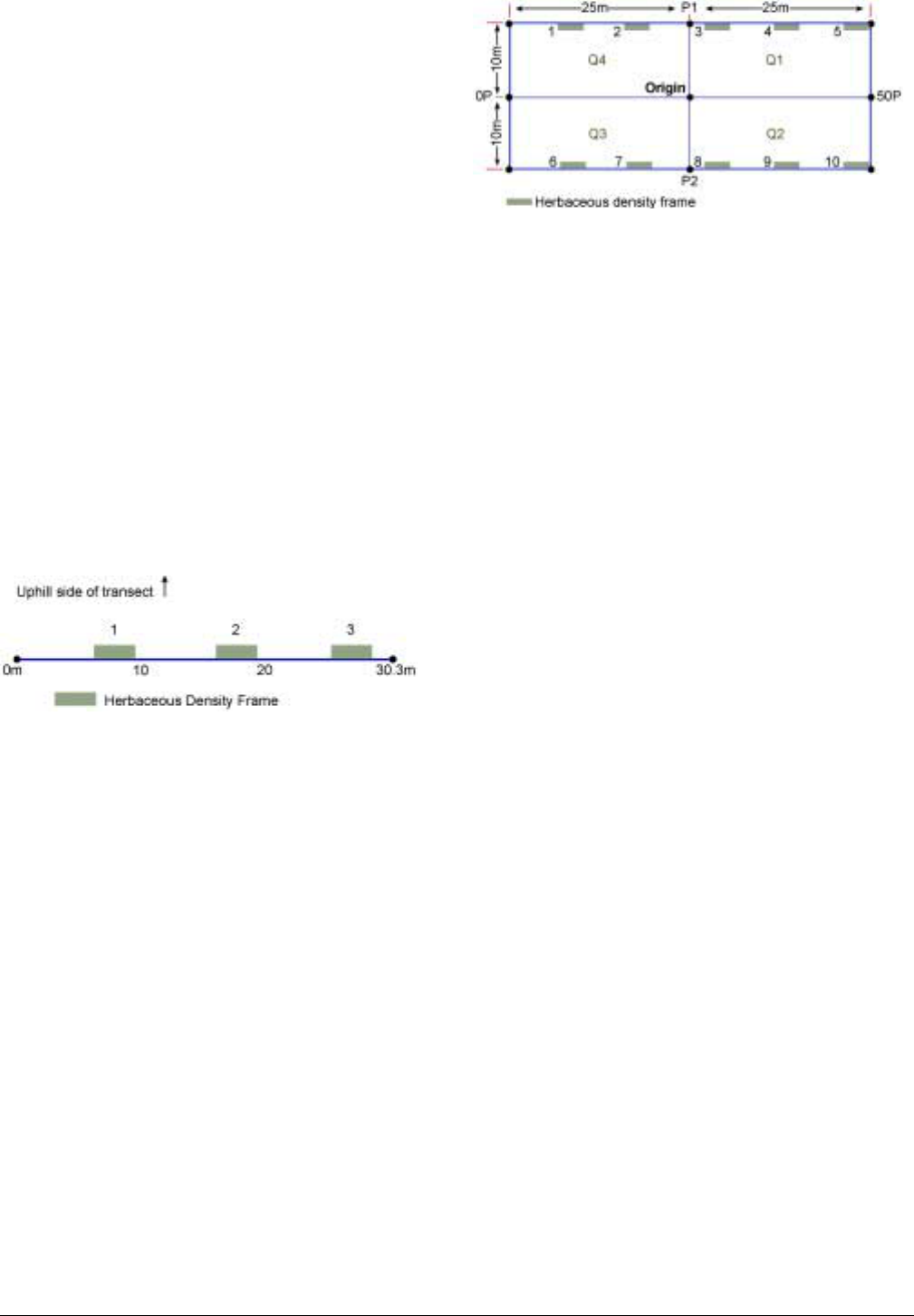
Optional Monitoring Procedures

Herbaceous layer species density

Grassland and brush plots—To measure the density

of forbs and/or grasses, place a frame (the size and

shape of which is determined during pilot sampling;

see page 47) on the uphill side of the shrub and herba-

ceous layer transect every 10 m (unless you are using a

belt transect because the vegetation is sparse). When it

is not clear which side of the transect is the uphill side,

use the right side of the transect when viewed from 0P

looking down the transect towards 30P. It is important

to record on the Herbaceous density data sheet (FMH-

18) which side of the transect you sampled so future

monitors will repeat your actions. The highest corner

of the first frame would be at the 10 m mark, there-

fore, sampling frame 1 would fall between 6 and 10 m

on the tape if you use a 0.25 × 4 m (1 m

2

) frame; the

next sampling areas would be between 16 and 20 m

(frame 2), and 26 and 30 m (frame 3) (see Figure 23).

The total area sampled using this example would be 3

m

2

. Record these density data on the Herbaceous den-

sity data sheet (FMH-18).

Figure 23. Density sampling frames (1 m

2

) for herbaceous

species in a grassland or brush plot.

Forest plots—For forest plots the procedure is the

same as for grassland and brush plots; the only differ-

ence is frame placement. Place the frame on the plot

side (interior) of the shrub and herbaceous layer

transect (Q4–30 m or Q4–Q1 and/or Q3–Q2) every

10 m (unless you are using a belt transect because the

vegetation is sparse). The highest corner of the first

frame would be at the 10 m mark; therefore, the first

sampling frame would fall between 6 and 10 m on the

tape if you use a 0.25 × 4 m (1 m

2

) frame; the next

sampling areas would be from 16 to 20 m (frame 2), 26

to 30 m (frame 3) (stop here for Q4–30 m plots), 36 to

40 m (frame 4), and 46 to 50 m (frame 5). Repeat this

process on the Q3–Q2 line in frame numbers 6–10, if

you are reading the Q3–Q2 line with the point inter-

cept transect (see Figure 24). The total area sampled

using the above example would be 10 m

2

(5 m

2

sam-

pled on each transect). Record these density data on

the Herbaceous density data sheet (FMH-18).

Figure 24. Density sampling frames (1 m

2

) for herbaceous

species in a forest plot.

Brush fuel load

Total biomass (fuel) and percent dead (live to dead

ratio) may be determined in brush types with sufficient

accuracy to make fire behavior predictions. When

required for smoke management, total brush biomass

must also be measured. Use standard biomass estimat-

ing techniques or existing species-specific estimating

equations to determine fuel load.

Brush biomass

Use standard biomass estimating techniques or exist-

ing biomass estimating equations to estimate the biom-

ass of each shrub in the plot. There are several other

methods to estimate biomass, height-weight curves,

capacitance meters, and double sampling; see Elzinga

and Evenden 1997 under the keyword biomass for an

excellent list of references, or review the references on

page 237 (Appendix G).

Percent dead brush

There are three techniques to estimate percent dead

brush: visual estimates; estimates based upon existing

publications such as a photo series; or direct measure-

ment of live-dead ratio using the following procedure:

• Randomly select a sample shrub of each species of

concern within a 1 acre area, outside of your mon-

itoring plot.

• Remove all branches 0.25 in or less in diameter,

and place in separate airtight bags according to

whether they are alive or dead. Take a subsample

of the shrub if the shrub is very large.

• Determine the net weight of the live portion and

the dead portion.

• Dry at 100°C.

• Determine oven dry weight of live portion and

dead portion. Use a subsample if necessary. If you

use a subsample, take care to weigh the sample

and subsample at the same time before drying.

• After determining the dry weights separately, cal-

culate the biomass in kilograms/hectare or tons/

Chapter 5 n

nn

n Vegetation Monitoring Protocols 89

acre for live and dead portions (see page 216,

Appendix D).

Grass biomass

When smoke management is a specific concern, or

hazard fuel reduction is the primary burn objective,

you need to estimate biomass. For information on

other methods see the note under “Brush Biomass”

above. Use this procedure to qualitatively determine

grass biomass:

Randomly toss a rigid quadrat of known area into the

plot. Do this six times. Each time:

• Clip all the vegetation to within 1 cm of the

ground.

• Place the clipped vegetation into paper bags. Each

quadrat should have one bag.

• Label each container with the plot identification

code, the bag number, and the collection date.

• Determine the sample dry weight by drying the

material in their bags until the weight stabilizes.

The oven temperature should be 100°C. Check

your samples 24 hours after they have been in the

oven.

• Calculate the kilograms/hectare or tons/acre for

each sample (see page 216, Appendix D).

Table 16. Accuracy standards for herbaceous (RS)

variables.

Herbaceous Layer

Herbaceous Density # of Individuals ± 5%

Shrub Density # of Individuals ± 5%

Herb Height ± 0.5 decimeters

Fire Monitoring Handbook 90

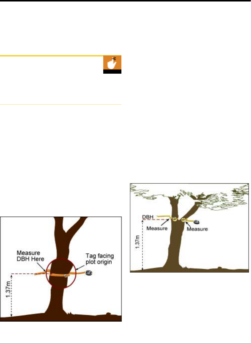
Monitoring Overstory Trees

Overstory trees are defined in this handbook as living

and dead trees with a diameter at breast height (DBH)

of >15 cm. Diameter at breast height is measured at

breast height (BH) 1.37 m (4.5 ft) from ground level.

You may modify this definition for your purposes; see

page 44 for details.

Overstory Tree Accuracy Standards

Accuracy standards for each variable discussed in this

section are listed at the end of this section (Table 21,

page 99).

TAG AND MEASURE ALL OVERSTORY

TREES

RS Procedures

Measure DBH for and tag all overstory trees within the

sampling area chosen during the monitoring design

process (see page 44). Check your protocols (FMH-4)

before proceeding. Living and dead trees are tagged

with sequentially numbered brass tags nailed into the

trees at BH (for each plot, use tag numbers different

from those used for the pole-size trees, e.g., 1-100 for

poles and 500-600 for overstory). Orient the tags so

that each faces the plot center (see Figure 25), except

in areas (e.g., near trails) where you will need to orient

the tags to make them less visually obtrusive.

Figure 25. DBH measurement and tag placement.

For a tree on a slope, determine the DBH while stand-

ing at the midslope side of the tree. Measure the DBH

of a leaning tree by leaning with the tree and measuring

perpendicular to the bole.

First, drive an aluminum nail into the tree at BH, so

that the tag hangs down and away from the tree and

several centimeters of nail remains exposed, leaving

ample space for tree growth.

Second, measure DBH (in centimeters) to the nearest

mm, just above the nail. Include trees on the plot

boundary line if >50% of their bases are within the

plot. Start in Quarter 1 and tag through Quarters 2, 3,

and 4 consecutively.

For non-sprouting tree species forked below BH, indi-

vidually tag and measure each overstory-size bole

(Figure 26). For sprouting tree species, tag and mea-

sure only the largest bole (in diameter) of the cluster.

For clonal tree species, e.g., aspen, treat each bole as an

individual tree. Tally seedling-size sprouts as resprout

class seedlings until they grow into the pole tree size

class. Note: If the main bole of a sprouting species has

died, but the tree is sprouting from the base, consider

the main bole dead.

Figure 26. DBH measurement for non-sprouting trees

forked below BH.

If the bole of a fallen tree is below BH, and the indi-

vidual is resprouting, treat the sprouting branches as

individuals and place them in the appropriate size class

(seedling, pole, or overstory). Include clarifying com-

ments on the data sheet, especially for resprouting

trees.

Chapter 5 n Vegetation Monitoring Protocols 91

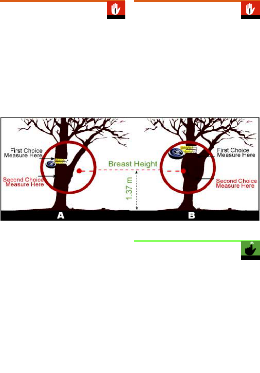
Sampling Problems with DBH

Note: The following tips are additions to this hand-

book; incorporate them with caution.

Swelling at BH If a swell or other irregularity occurs

at the standard 1.37 m height for DBH, place the tag

above or below the swell and DBH measured at the

tag. Make every attempt to keep the tag (and thus the

DBH measurement) between 1 and 2 m above the

ground, trying above the obstruction first. If you do

not measure DBH at BH, note this on the data sheet

(Comments) (See Figure 27).

Void at BH

If you find a void caused by a fire scar or other abnor-

mality, and a large part of the bole is missing at BH,

and it would be impractical to simply measure above or

below it, it may be necessary to estimate what the

DBH would be, were the bole intact. If this is done, be

sure to note in the comments field that the DBH was

estimated (See Figure 28).

Figure 27. Handling irregularities at BH.

A) a tree with a branch at BH, B) a tree with a swell at BH.

Measure DBH

Wrap a diameter tape (not a standard tape) around the

tree in the plane of the nail, making sure the tape does

not sag, and read the diameter. Take care to read at the

measurement line, not at the end of the tape. Record

the heading information on Overstory tagged tree data

sheet (FMH-8 in Appendix A). For all overstory trees,

record the plot quarter in which the tree occurs (Qtr),

the tree tag number (Tag), species (Spp), and diameter

(DBH), and circle whether the tree is alive. Record

miscellaneous overstory tree information in Com-

ments. Map each overstory tree by tag number on the

appropriate tree map (FMH-11, -12, -13, or -14).

Measuring DBH without a Diameter

Tape

If you do not have (or have forgotten) a diameter tape,

you can use a standard tape to measure circumference,

and then calculate diameter as follows:

circumference

DBH= --------------------------------------

π

Fire Monitoring Handbook 92

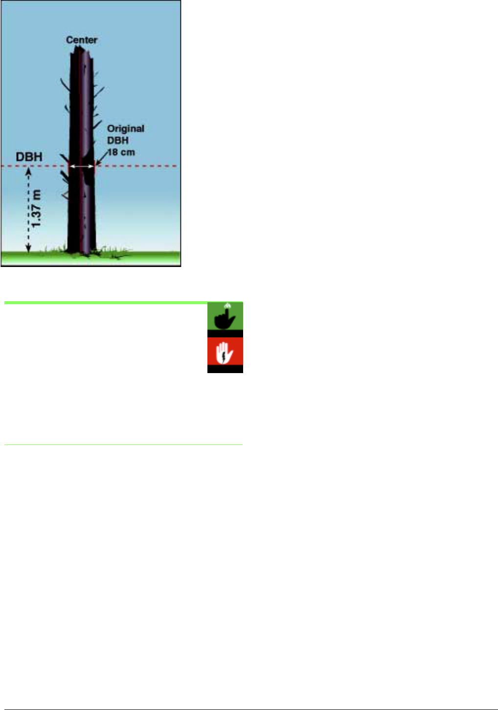
for dead and down or completely consumed (CPC 10),

(B) for broken below DBH (CPC 11), and (S) for cut

stump (CPC 12). Note that these three codes are used

only once during data collection.

Figure 28. Reconstruct DBH when it would provide a better

estimate of the regular bole of the tree.

Toxic Plants at DBH

If toxic plants embrace the bole at BH, carefully place

the tag at an appropriate location. It may also be

acceptable to estimate DBH in some cases, after con-

sultation with resource and fire specialists.

OPTIONAL MONITORING PROCEDURES

Crown Position and Tree Damage

If possible, also monitor the optional variables crown

position (CPC) and tree damage (Damage). Space is

provided on the FMH-8 data sheet for these data.

Crown position

Crown position, an assessment of the canopy position

of live overstory trees (Avery and Burkhart 1963), is

recorded in the column marked CPC (crown position

code) using a numeric code (1–5) (see Table 17,

page 94 and Figure 29, page 94). Codes for dead trees

(Thomas and others 1979) can also be recorded using

numeric snag classes (6–12) (see Table 18, page 95 and

Figure 30, page 95).

During the immediately postburn visit use the “Live”

column on FMH-20 for CPC codes (10–12). Use (C)

Chapter 5 n Vegetation Monitoring Protocols 93

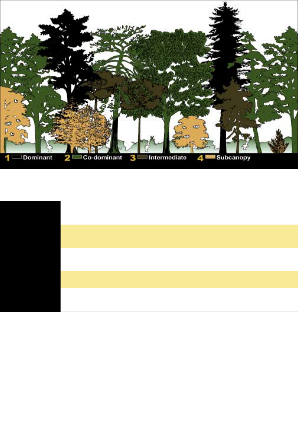
Figure 29. Crown position codes for live trees.

A fifth code (5) is used for isolated trees.

Table 17. Descriptions of live tree crown position codes.

1 Dominant

2 Co-dominant

3 Intermediate

4 Subcanopy

5 Open Growth/

Isolated

Trees with crowns extending above the general level of the crown cover, and receiving full light from

above and at least partly from the side; these trees are larger than the average trees in the stand and

have well-developed crowns, but may be somewhat crowded on the sides.

Trees with crowns forming the general level of the crown cover and receiving full light from above, but

comparatively little from the sides; these trees usually have medium-size crowns, and are more or less

crowded on the sides.

Trees shorter than those in the two preceding classes, but with crowns either below or extending into the

crown cover formed by co-dominant and dominant trees, receiving little direct light from above, and none

from the sides; these trees usually have small crowns and are considerably crowded on the sides.

Trees with crowns below the general level of the crown cover and receiving no direct light from above or

from the sides.

Trees receiving full sunlight from above and all sides. Typically, these are single trees of the same gen-

eral height and size as other trees in the area, but where the stand is open and trees are widely sepa-

rated so dominance is difficult to determine.

Fire Monitoring Handbook 94

Figure 30. Crown position codes for dead trees.

Table 18. Descriptions of dead tree crown position codes.

6 Recent Snag

7 Loose Bark

Snag

8 Clean Snag

9 Broken Above

BH

10 Broken Below

BH

11 Dead and Down

12 Cut Stump

Trees that are recently dead with bark intact. Branches and needles may also be intact.

Trees that have been dead several years on which the bark is partially deteriorated and fallen off; tops

are often broken.

Trees that have been dead several years with no bark left. Usually most of the branches will be gone as

well; tops are often broken.

Trees that have been dead a long time with no bark, extensive decay, and that are broken above BH.

Postburn trees that extended above BH preburn, but no longer do. Note: Only record data for a tree the

first time you find it broken.

Postburn trees that stood preburn and have since fallen or been consumed. Note: Only record data for

a tree the first time you find it down.

Postburn trees that stood preburn and has been cut as a result of fire operations. Note: Only record

data for a tree the first time you find the stump.

Chapter 5 n Vegetation Monitoring Protocols 95

Crown Position Codes (CPC)

Earlier editions of the Fire Monitoring Handbook

(USDI NPS 1992) used only the first four crown posi-

tion codes. For plots established earlier, there is no

harm in adopting this new protocol and assigning

codes to snags after plots have burned. As plots are

revisited according to their normal schedule, previ-

ously dead trees should be assessed for their snag

codes. An effort can also be made to determine what

the code might have been at the previous visits. For

example, a clean snag (CPC 8) encountered during the

year-2 visit was probably a clean snag at year-1, and

possibly even at preburn. Any estimated data should be

added to the database retroactively for those previous

visits along with a comment noting that the CPC is a

guess. In many cases a comment might have been

made as to the status of the snag during the past visit.

Data Collection on Trees with a CPC of

10–12

Only collect data for trees that are newly fallen, con-

sumed, cut, or broken below BH (CPC 10–12) the first

time you encounter them after the preburn visit.

Never record a dead and down, cut, or broken below

BH tree during the preburn visit. Once you record data

for a newly fallen, consumed, broken, or cut tree,

ignore it in your tree density data collection from that

point onward. For example, if you find a tree with a

CPC of 11 during the immediate postburn visit, for

your year-1 re-measurement of that plot you would not

record any data for that tree.

Immediate postburn—See page 111 under “Scorch

Height.”

Year-1 postburn and beyond—For a dead tree with a

CPC of 10–12 that you encounter in year-1 and

beyond, you only need to record data for that tree

once. For example, a tree’s bole breaks off below BH

between the year-1 and year-2 plot visits. You would

assign this tree a CPC of 10 in the year-2 visit, and then

in subsequent visits you would not record any data for

that tree.

Tree damage

You may wish to identify living overstory trees exhibit-

ing signs of stress (loss of vigor) before the burn. By

doing this you can infer that if those trees die relatively

soon following the fire, their death may not be wholly

attributable to the fire, but to a combination of factors.

The monitor’s ability to evaluate preburn damage will

determine the value of the data. A trained specialist

will undoubtedly observe more than a novice in the

field. Note: Appendix G contains several forest pest

and disease references; see page 229.

The following list (Table 19) of structural defects and

signs of disease is simplistic (and certainly not all-inclu-

sive), but should serve as a useful guideline. Parks may

add categories to include damage of local importance

in the “Comments” column. Record these data for liv-

ing overstory trees (tree damage assessment is optional

for dead trees) under Damage on the FMH-8 form in

Appendix A.

Table 19. Damage codes for overstory trees.

ABGR

BIRD

BLIG

BROK

BROM

BURL

CONK

CROK

DTOP

EPIC

EPIP

FIRE

Abnormal growth pattern for the species of con-

cern. This category would include a range of

physical deformities not included in the remain-

der of the damage codes.

Bird damage such as woodpecker or sapsucker

holes.

Blight is generally defined as any plant disease

or injury that results in general withering and

death of the plant without rotting. Blight can result

from a wide variety of needle, cone, and stem

rusts, as well as canker diseases, and is often

species- or genus-specific. Consultation with

local plant pathologists may assist in identifying

specific blight conditions.

Broken top of the tree.

Witches’ broom diseases are characterized by an

abnormal cluster of small branches or twigs on a

tree as a result of attack by fungi, viruses, dwarf

mistletoes, or insects. Brooms caused by dwarf

mistletoe and from yellow witches’ broom dis-

ease are common in the west.

A hard, woody, often rounded outgrowth on a

tree. This occurs naturally in some tree and

shrub species, and is a sign of an infection or dis-

ease in other species.

The knobby fruiting body of a tree fungal infection

visible on a tree bole, such as a shelf fungus.

Crooked or twisted bole for species in which this

is uncharacteristic.

Dead top.

Epicormic sprouting, adventitious shoots arising

from suppressed buds on the stem; often found

on trees following thinning or partial girdling.

Epiphytes present.

Fire scar or cambial damage due to fire.

Fire Monitoring Handbook 96

Table 19. Damage codes for overstory trees. (Continued)

FORK

FRST

GALL

HOLW

INSE

LEAN

LICH

LIGT

MAMM

MISL

MOSS

OZON

ROOT

ROTT

SPAR

SPRT

TWIN

UMAN

WOND

Forked top of a tree or multiple primary leaders in

a tree crown for species in which this is unchar-

acteristic. Forks assume vertical growth and

should be distinguished from branches, which

assume horizontal growth.

Frost crack or other frost damage.

Galls found on stems, leaves or roots. Galls are

formed by infection of the plant by bacteria or

fungi, or by an attack by certain mites, nema-

todes, or insects, most notably wasps.

Hollowed-out trees. Repeated hot fires can burn

through the bark and the tree’s core may then rot

out, especially in trees with tough bark, but soft

heartwood, e.g., sequoia, coast redwood. These

hollowed-out trees are sometimes called “goose

pens” because early settlers kept poultry in them.

Visible insects in the tree bole or the canopy, or

their sign, such as frass, pitch tubes or bark bee-

tle galleries.

Tree is leaning significantly. If on a slope, tree

deviates considerably from plumb.

Lichens present.

Lightning scar or other damage to the tree

caused by lightning.

Damage caused by mammals, such as bear claw

marks, porcupine or beaver chewings, and deer

or elk rubbings.

Mistletoe is visible in the tree (as opposed to

signs of mistletoe, such as broom, without visible

mistletoe).

Moss present.

Ozone damage. Ozone injury is often seen in the

form of stippling or speckling on the leaves or

needles of trees. This discoloration varies among

species and ranges in color from red or purple to

yellow or brown. Susceptible species often drop

their leaves prematurely.

Large exposed roots.

A rot of fungus other than a conk, often associ-

ated with a wound or crack in a tree.

Unusually sparse foliage for that species and

size of tree.

Basal sprouting; new shoots arising from the root

collar or burl.

A tree that forks below BH and has two or more

boles. Use this code for tree species that typically

have single boles.

Human-caused damage such as axe marks,

embedded nails or fence wire, or vandalism.

A wound to a tree that cannot be identified by

one of the other damage codes, including

wounds or cracks of unknown cause.

Damage Codes

Some damage codes may not be applicable to all spe-

cies. For example, some species of oak are character-

ized by complex forking above BH, so the FORK code

would not indicate damage or abnormality and would

not be of use.

If several types of insect damage are present, it may be

desirable to distinguish among them in the comments

field on the FMH-8.

After the initial preburn data collection visit, you may

find it advantageous to copy the damage codes, crown

position codes and comments from the previous visit’s

tagged tree data sheet to the current visit’s data sheet.

This will encourage consistency between visits and

minimizes the risk of one data collector seeing some-

thing like mistletoe one year, the next year’s data collec-

tor missing it and the subsequent visit’s collector seeing

it again, leading to the erroneous assumption that it has

actually come and gone. Note: Document any damage

noted in past years that you could not find.

Measuring Diameter at Root Crown (DRC) for

Woodland Species

Measurement of a tree’s diameter at root crown is an

alternative to DBH measurements for tree species that

are typically highly forked. Note: Do not use this

method for unusual individual trees that have many

boles. With this method, trees with stems that fork

underground, or with several stems clumped together

that appear to be from the same root origin, are treated

as a single tree. The single diameter of the root crown

should be measured directly if branching occurs above

ground and the single diameter accurately reflects the

cumulative volume of the stems it supports. Alterna-

tively, if the stems fork below ground level, or the base

is deformed and its diameter would grossly overesti-

mate the volume of the individual stems, the DRC

should be calculated from the individual stem diame-

ters (see page 214, Appendix D for this equation).

To measure a single stem, or each of multiple stems

forked underground, carefully remove the loose mate-

rial to the mineral soil (remember to replace it when

finished) at the ground line or stem root collar, which-

ever is higher. Measure DRC just above any swells

present, and in a location such that the diameter mea-

surements are reflective of the volume above the

stems. For measurement of multiple stems, forked

Chapter 5 n Vegetation Monitoring Protocols 97

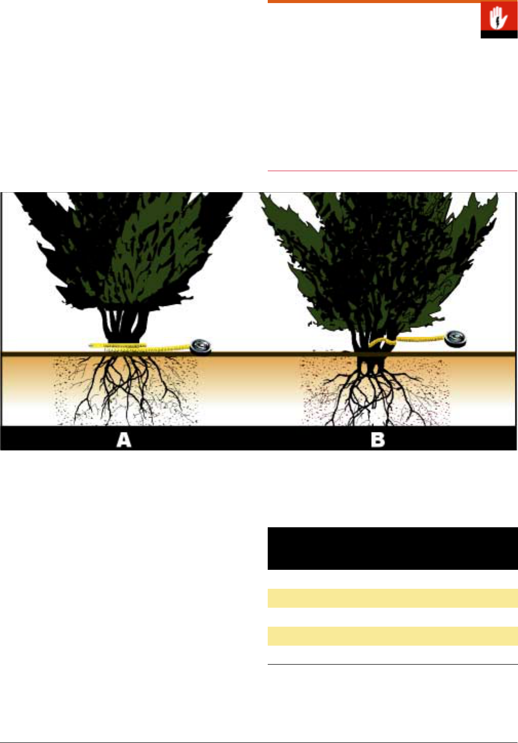
above ground, measure DRC just above the fork, and

above any swells (see Figure 31).

Diameter at Root Crown

Where a stem is missing or damaged, estimate what its

diameter would have been. If a stem is now dead, but

previously contributed to the crown, count it. Individ-

ual stems must be (or have been prior to damage) at

least 1.37 m tall and must have a DRC of at least 2.5

cm to qualify for measurement.

Attach a tag (optional) to the largest or main stem, fac-

ing the plot origin and approximately one foot above

ground level.

Diameter at root crown is a new addition to the hand-

book with this edition. Resource and fire managers

may determine that it would be a more useful measure

for a given species than diameter at breast height

(DBH). If this is the case, then both methods should

be used for a minimum of two years, or until a correla-

tion between DBH and DRC can be established for

that species at that site.

Figure 31. Measuring multiple stems forked above ground with DRC.

Measure just above the fork, and above any swells. Measurement of: A) multiple stems forked above ground, B) single stems, or stems

forked underground.

Diameter Groupings

Overstory trees.

This includes single-stemmed trees

>15 cm DRC and multi-stemmed trees with a cumula-

tive DRC >15 cm (though you can modify this defini-

tion; see page 44).

Pole-size trees.

This includes single-stemmed trees

between 2.5 cm and 15 cm DRC, and multi-stemmed

trees with a cumulative DRC between 2.5 cm and 15

cm (though you can modify this definition; see page

44).

For trees with several small stems, the following guide-

lines (Table 20) may help in determining whether a tree

will qualify as an overstory tree (if there is any ques-

tion, measure the stems).

Table 20. Guidelines to determine whether a tree is

considered an overstory tree.

Approximate Stem Size

(cm)

Approx. Number of Stems

Needed to Exceed 15.0

cm DRC

10.5 2

8.5 3

5.0 9

3.5 18

2.5 35

Fire Monitoring Handbook 98

Table 21. Accuracy standards for overstory tree (RS)

variables.

Overstory Tree

DBH/DRC 15.1–50 cm + 0.5 cm

51–100 cm + 1 cm

>100 cm Not Applicable

Tree Damage Best Judgment

Crown Position Best Judgment

# of Individuals ± 5%

Chapter 5 n Vegetation Monitoring Protocols 99

Monitoring Pole-size Trees

Pole-size trees are defined in this monitoring system as

standing living and dead trees with a diameter at breast

height (DBH) >2.5 cm and <15 cm. You may modify

this definition for your purposes; see page 44 for

details.

Pole-size Tree Accuracy Standards

Accuracy standards for each variable discussed in this

section are listed at the end of this section (Table 23,

page 101).

MEASURE DENSITY AND DBH OF POLE-

SIZE TREES

RS Procedures

Count and measure DBH for all pole-size trees within

the sampling area chosen during the monitoring design

process (see page 45). Check your protocols (FMH-4)

before proceeding.

Tagging pole-size trees is optional. If you choose to tag

pole-size trees, for each plot be sure to use numbers

different from those used for overstory trees, e.g., 1-

100 for poles and 500-600 for overstory. The proce-

dure is as for overstory trees: drive an aluminum nail

into each tree at BH so that the tag hangs down and

away from the tree and several centimeters of nail

remain exposed, leaving ample space for tree growth.

Second, measure DBH (in centimeters) to the nearest

mm, just above the nail. When the tree is too small to

tag at BH, or the tagging nail could split the trunk,

place the tag at the base of the tree.

On the Pole-size tree data sheet (FMH-9) record the

quarter in which the tree occurs (Qtr), tag or map

number, the species (Spp), the diameter (DBH) of each

tree, and whether it is alive (Live).

For non-sprouting tree species forked below BH, indi-

vidually tag and measure each pole-size bole. For

sprouting tree species, tag and measure only the largest

bole (in diameter) of the cluster. Remember that if the

largest bole has a DBH of >15 cm, the tree is an over-

story tree. Tally seedling-size sprouts as resprout class

seedlings until they grow into the pole tree size class.

Note: If the main bole of a sprouting species has died,

but the tree is sprouting from the base, consider the

main bole dead.

If the bole of a fallen tree is below BH, and the indi-

vidual is resprouting, treat the sprouting branches as

individuals and place them in the appropriate size class

(seedling, pole, or overstory). Include clarifying com-

ments on the data sheet, especially for resprouting

trees.

For trees with swellings or voids at BH, refer to page

92 in the overstory tree section.

If you do not individually tag trees, you can assign a

map number for each tree, or simply count them by

species (and height class, if desired). Finally, map each

tree using a map (or tag) number on the appropriate

tree map (FMH-11, -12, -13, or -14).

OPTIONAL MONITORING PROCEDURES

Measuring Diameter at Root Crown for Woodland

Species

Measurement of a tree’s diameter at root crown (DRC)

is an alternative to DBH measurement for tree species

that are typically highly forked. This method is pre-

sented in the Overstory Tree section (page 97).

Measure Pole-size Tree Height

If you choose to measure this optional dataset, mea-

sure and record pole-size tree height (Hgt) on the

Pole-size tree data sheet (FMH-9) for each tree

encountered. Use height class codes five through 13

(Table 22, also available for reference on FMH-9).

Fire Monitoring Handbook 100

Table 22. Height class codes for pole-size trees.

A tree must be breast height (1.37 cm) or taller to be classified as pole-size.

Code Height (cm) Code Height (cm) Code Height (cm) Code Height (cm)

1 0–15 5 100.1–200 9 500.1–600 13 900.1+

2 15.1–30 6 200.1–300 10 600.1–700

3 30.1–60 7 300.1–400 11 700.1–800

4 60.1–100 8 400.1–500 12 800.1–900

Note: Measure height from ground level to the highest point of growth on the tree. The highest point on a bent tree would be down

the trunk of the tree instead of at the growing apex Only use height codes 1-4 for leaning trees.

Table 23. Accuracy standards for pole-size tree (RS)

variables.

Pole Tree

DBH/DRC + 0.5 cm

Pole Height Within Class

Number of Indi- ± 5%

viduals

Chapter 5 n Vegetation Monitoring Protocols 101

Monitoring Seedling Trees

Seedling trees are defined in this monitoring system as

living trees with a diameter at breast height (DBH)

<2.5 cm (recording information on dead seedlings

is optional). Trees that are less than the height

required for DBH are treated as seedlings, regardless

of age and diameter. By definition, a tree cannot be

pole-size and less than the height necessary for DBH.

You may modify this definition for your purposes; see

page 44 for details. Note: Accuracy standards for each

seedling tree variable are listed in Table 24.

Table 24. Accuracy standards for seedling tree (RS)

variables.

Seedling Tree

DBH <2.5 cm No Errors

Seedling Height Within Class

# of Individuals ± 5%

COUNT SEEDLING TREES TO OBTAIN

SPECIES DENSITY

Count the number of seedling trees by species within

the sampling area chosen during the monitoring design

process (see page 45). Check your protocols (FMH-4)

before proceeding.

RS Procedures

Record the heading information on the Seedling tree

data sheet (FMH-10 in Appendix A). For all seedling

trees, record the number of individuals (Num) by spe-

cies (Spp) on the FMH-10. An optional sketch map of

the seedling tree aggregates may be made on any tree

map (FMH-11, -12, -13, or -14). In areas with few

seedlings in the understory or where tracking individ-

ual seedlings through time is important, an optional

Table 25. Height class codes for seedling trees.

mapping procedure is to give individual seedlings

sequential map numbers (Map#), so that data can be

correlated between the Seedling tree data sheet (FMH-

10) and the appropriate tree map (FMH-11, -12, -13,

or -14). On the data sheet, indicate whether each

group of tallied trees is alive or dead (Live) or a

resprout (Rsprt).

Seedling Resprout Class

Seedlings can now be classed as resprouts. See page

255 in the Glossary for a definition.

Anticipated dramatic increases in postburn

seedling density

The seed banks of some tree species may germinate

profusely following a burn. Rather than count thou-

sands of seedlings, it may be more efficient to subsam-

ple the plot during temporary high density periods. To

subsample, grid the sample area listed on your FMH-4

and randomly select an appropriate subsample (i.e.,

10%, 20%) of the area. Then proceed to count the

individuals in the subsample area and extrapolate to

the full sample area listed on your FMH-4. Again, this

should only be done in consultation with resource and

fire managers.

OPTIONAL MONITORING PROCEDURES

Measure Seedling Tree Height

Record the number of seedling trees (Num) by species

(Spp) in each height class (Hgt) on the Seedling tree

data sheet (FMH-10) for each tree encountered. Use

the following height class codes (Table 25, also avail-

able for reference on FMH-10):

Code Height (cm) Code Height (cm) Code Height (cm) Code Height (cm)

1 0–15 5 100.1–200 9 500.1–600 13 900.1+

2 15.1–30 6 200.1–300 10 600.1–700

3 30.1–60 7 300.1–400 11 700.1–800

4 60.1–100 8 400.1–500 12 800.1–900

Note: Measure height from ground level to the highest point of growth on the tree. The highest point on a bent tree would be down

the trunk of the tree instead of at the growing apex.

Fire Monitoring Handbook 102

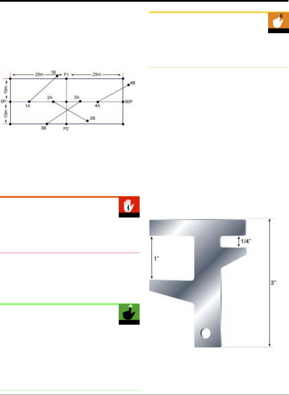
nitoring Dead and Downed Fuel Load

Monitoring Dead & Downed Fuel Load

On all forest monitoring plots, measure dead and

detached woody fuel as well as duff and litter depths.

These measurements are taken along fuel inventory

transects, which must be relocatable to allow evalua-

tion of postburn fuel load. Transects extend in random

directions originating from the centerline at 10, 20, 30,

and 40 m (Figure 32).

Figure 32. Location of fuel inventory transects.

Unlike herbaceous transects, fuel load transects can

cross each other (Brown 1996). In many monitoring

types the transect length is 50 ft, but in types with

sparser fuels it may exceed that (see page 45). Check

your protocols (FMH-4) before proceeding.

Fuel Load Measurements

Fuel load measurements and the transects used to

sample them traditionally use English measurements,

not metric.

Lay out the appropriate length tape along the transect

in a random direction (Appendix B). Place a labeled

tag at each end of the transect (see page 70 for a

description of how to label tags). Measure the percent

slope of the transect (from end to end) in percent.

When an Obstruction is Encountered

Along the Fuel Transect

If the fuel transect azimuth goes directly through a

rock or stump, in most cases you can run the tape up

and over it. If the obstruction is a tree, go around it

and pick up the correct azimuth on the other side. Be

sure to note on the FMH-19 on which side of the bole

the tape deviated so that it will be strung the same way

in the future.

Fuel Load Accuracy Standards

Accuracy standards for each variable discussed in this

section are listed at the end of this section (Table 27,

page 105).

RS PROCEDURES

Working along the distances defined in the monitoring

type protocols (FMH-4), tally each particle intersected

along a preselected side of the tape, categorized by size

class. A go-no-go gauge with openings (0.25, 1, and 3

in) works well for separating borderline particles into

size classes and for training the eye to recognize these

size classes (Figure 33). Measurement of all particles is

taken perpendicular to the point where the tape

crosses the central axis (Figure 34, page 104). Count

intercepts along the transect plane up to 6 ft from the

ground. Count dead and down woody material, but

not cones, bark, needles and leaves. Do not count

stems and branches attached to standing shrubs or

trees (Brown 1974; Brown and others 1982). For addi-

tional details on tallying downed woody material, refer

to the notes on the reverse side of FMH-19.

Figure 33. Graphic of a go-no-go gauge.

Chapter 5 n Vegetation Monitoring Protocols 103

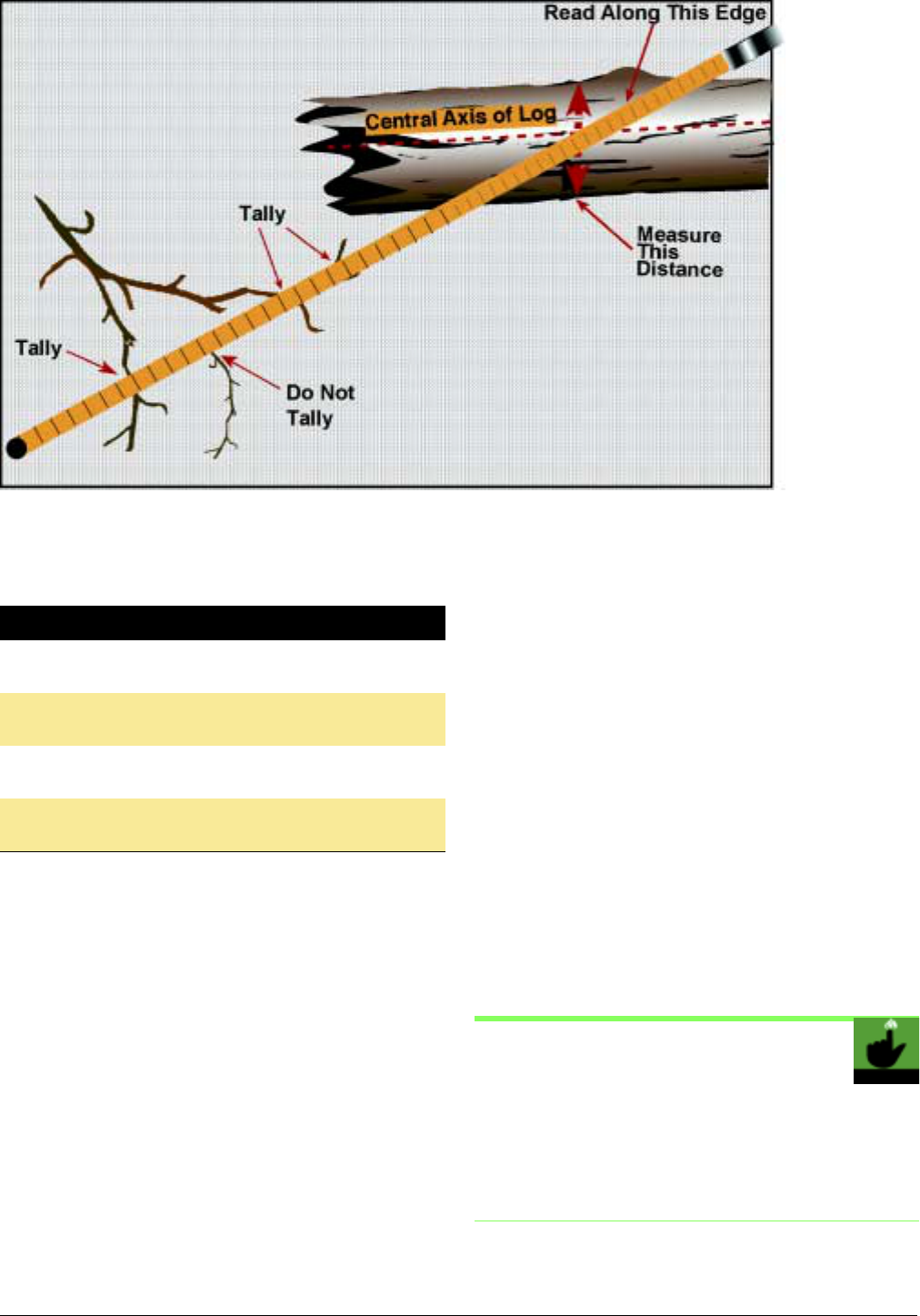
Figure 34. Tally rules for dead and down fuel.

Count all intersections, even curved pieces. All intersections must include the central axis in order to be tallied.

Table 26. Suggested lengths of transect lines to tally fuels

by size class.

Size Class Suggested Length

0–0.25” (0–0.62 cm) tally from 0–6 ft

diameter (1 hour)

0.25–1” (0.62–2.54 cm) tally from 0–6 ft

diameter (10 hour)

1–3” (2.54–7.62 cm) tally from 0–12 ft

diameter (100 hour)

>3” (>7.62 cm) measure each log

diameter (1,000 hour) from 0–50 ft

Differentiate between 3 in (or larger) diameter parti-

cles that are sound and those that are rotten. Rotten

wood is that which is obviously deteriorating or punky.

Measure the particle diameter to the nearest 0.5 in with

a diameter tape or ruler. Ignore particles buried more

than halfway into the duff at the point of intersection.

Visually reconstruct rotten logs as a cylinder and esti-

mate the diameter. This reconstructed diameter should

reflect the existing wood mass, not the original sound

diameter.

Take depth measurements for litter and duff (as

defined in the Glossary) at 10 points along each fuel

transect—that is at 1, 5, 10, 15, 20, 25, 30, 35, 40, and

45 ft. If the transect is longer than 50 ft, do not take

additional litter and duff measurements. Do not take

measurements at the stake (0 point); it is an unnatural

structure that traps materials. At each sampling point,

gently insert a trowel or knife into the ground until you

hit mineral soil, then carefully pull it away exposing the

litter/duff profile. Locate the boundary between the

litter and duff layers. Vertically measure the litter and

duff to the nearest tenth of an inch. Refill holes created

by this monitoring technique. Do not include twigs

and larger stems in litter depth measurements.

You may choose to install duff pins to measure duff

reduction instead of digging and measuring the depth

of holes. Duff pins, however, are easy to trip over or

pull out, and therefore should be used only where traf-

fic (human or other animal) is limited.

Record the above dead and downed fuel data on the

Forest plot fuels inventory data sheet (FMH-19, in

Appendix A).

Measuring Duff and Litter

You can dig and measure in one step if you engrave or

etch a ruler in tenths of inches on the back of your

trowel. Use paint or nail polish to mark the major gra-

dations.

Fire Monitoring Handbook 104

DEAL WITH SAMPLING PROBLEMS

Occasionally moss, a tree trunk, stump, log, or large

rock will occur at a litter or duff depth data collection

point. If moss is present, measure the duff from the

base of the green portion of the moss. If a tree, stump

or large rock is on the point, record the litter or duff

depth as zero, even if there is litter or duff on top of

the stump or rock. If a log is in the middle of the litter

or duff measuring point, move the data collection

point 1 ft over to the right, perpendicular to the sam-

pling plane.

Table 27. Accuracy standards for fuel (RS) variables.

Fuel Load

% Slope ± 5%

Diameter of >3” logs ± 0.5 in (1.2 cm)

Litter or Duff Depth ± 0.5 in (1.2 cm)

Chapter 5 n Vegetation Monitoring Protocols 105

3

Monitoring Fire Weather And Behavior Characteristics

Monitoring Fire Weather & Behavior Characteristics

Collecting Fire Behavior and Weather

Data

Previous editions of the Fire Monitoring Handbook

(USDI NPS 1992) recommended that monitors record

fire weather and behavior characteristics at each plot

using Fire Behavior Observation Circles (FBOC) or

Intervals (FBOI). The revised recommendations fol-

low.

For the monitoring plots to be representative, they

must burn under the same conditions and ignition

techniques used in the rest of the prescribed fire block.

Fire monitor safety, however, must always be fore-

most.

Forest monitoring types may include a dense under-

story layer, while brush and grassland fuel types are

usually flashy; all of them may be unsafe to move

through during a fire. The monitoring procedure pre-

sented here is an ideal and will be impossible to imple-

ment in some situations. The objective of monitoring

fire characteristics in forest, brush or grassland types,

therefore, is to do whatever is necessary to be safe

while simultaneously obtaining representative fire

behavior measurements wherever possible.

Take fire weather and behavior observations (rate of

spread, flame length, and flame depth (optional), and

other level 2 variables described in Chapter 2) in the

same monitoring types represented by your plots, in an

area where the fire behavior is representative of fire

behavior on the plots. Where safe, you can make fire

behavior observations near a monitoring plot.

Fire Behavior Accuracy Standards

Accuracy standards for each variable discussed in this

section are listed in Table 29, page 111.

RATE OF SPREAD

To estimate Rate of Spread (ROS), you can use a Fire

Behavior Observation Interval (FBOI). An FBOI con-

sists of two markers placed a known distance apart,

perpendicular to the flame front. Five feet is a standard

length for the FBOI; however, you may shorten or

lengthen the FBOI to accommodate a slower or faster

moving flame front.

If you expect an irregular flaming front, set up another

FBOI, perpendicular to the first FBOI. That way you

will be prepared to observe fire behavior from several

directions. If the fire moves along either FBOI, or

diagonally, you can calculate ROS, because several

intervals of known length are available. To distribute

the FBOIs, use a setup that you think makes sense for

your situation.

As the fire burns across each FBOI, monitor the rec-

ommended Fire Conditions (level 2) variables, and

record observations on the Fire behavior–weather data

sheet (FMH-2, in Appendix A). The time required for

the fire to travel from one marker to the other divided

by the distance (5 ft) is recorded as the observed rate

of spread. For further information on ROS, see page

13.

Rate of Spread

You may use metric intervals to measure ROS. How-

ever, a possible problem with using metric ROS inter-

vals is that you may forget to convert the metric into

English units to get a standard linear expression for

ROS, which is chains per hour or feet per minute. To

avoid potential errors, it may be better to pre-measure

and mark the ROS intervals in feet.

FLAME LENGTH AND DEPTH

During the fire, estimate flame length (FL) and flame

depth (FD; optional) (see page 13) at 30-second inter-

vals (or more frequently if the fire is moving rapidly),

as the flaming front moves across the ROS observa-

tion interval. Use the Fire behavior–weather data sheet

(FMH-2) to record data. If possible, make five to ten

observations of FL and FD per interval. Note: Where

close observations are not possible, use the height (for

FL) or depth (for FD) of a known object between the

observer and the fire behavior observation interval to

estimate average flame length or flame depth.

Fire Monitoring Handbook 106

Fire weather observations should be recorded at 30-

minute intervals. Sample more frequently if you detect

a change in wind speed or direction, or if the air tem-

perature or relative humidity seems to be changing sig-

nificantly, or if directed to do so by the prescribed

burn boss.

Fireline Safety

• For safety, inform all burn personnel at the preburn

briefing that the unit contains monitoring plots. It is

recommended that you provide a brief discussion on

the value of these plots, and your role on the burn.

• Inform all ignition personnel that they are to burn as

if the plots do not exist. This will help avoid biased

data, e.g., running a backing fire through a plot while

using head fires on the rest of the unit.

Chapter 5 n Vegetation Monitoring Protocols 107

Monitoring Immediate Postburn Vegetation & Fuel Characteristics

GRASSLAND AND BRUSH PLOTS MONITOR POSTBURN CONDITIONS

After the burned plot has cooled sufficiently (generally Burn Severity—All Plot Types

within two to three weeks), remeasure the RS variables

(see Tables 5 and 6 on page 57). Record postburn con-

ditions that characterize the amount of heat received in

the type on the Brush and grassland plot burn severity

data sheet (FMH-22). On each form, circle the post-

burn status code as “01 Post” (within two months of

the burn, see tip box below). The first number repre-

sents the number of treatment iterations, e.g., 02 Post

would indicate that the plot had been burned (or oth-

erwise treated) twice.

FOREST PLOTS

After the burned plot has cooled sufficiently (generally

within two to three weeks), remeasure the RS variables

(see Table 7 on page 57) using the preburn monitoring

techniques. Record postburn conditions that charac-

terize the amount of heat received in the type on the

Forest plot burn severity data sheet (FMH-21). Remea-

sure the overstory and record data on the Tree post-

burn assessment data sheet, FMH-20 (optional for

pole-size trees). Do not remeasure the diameter of

overstory trees for at least one year postburn, but at

every visit record whether each tree is alive or dead.

On each form, circle the postburn status code as “01

Post” (within two months of the burn). The first num-

ber represents the number of treatment iterations, i.e.,

02 Post would indicate that the plot had been burned

(or otherwise treated) twice.

Timing Burn Severity Data Collection

You can lose burn severity data by waiting too long to

collect it, and having rain or snow mar the data collec-

tion. Collect burn severity data as soon as possible

after the plot cools, which can be much less time than

the recommended two weeks, especially in grasslands.

Immediate Postburn Vegetation & Fuel

Characteristics Accuracy Standards

Accuracy standards for each variable discussed in this

section are listed at the end of this section (Table 29,

page 111).

Visual assessments of burn severity allow managers to

broadly predict fire effects upon the monitoring type,

from changes in the organic substrate to plant survival

(Ryan and Noste 1985). Burn severity is rated and

coded separately for organic substrate and vegetation,

distinguished by an S or V, respectively. Rate burn

severity according to the coding matrix (Table 28,

page 110; adapted from Conrad and Poulton 1966;

Ryan and Noste 1985; Bradley and others 1992).

Example:

In a plant association dominated by shrubs you

observe the following conditions at one of the 4 dm

2

burn severity data collection points: the leaf litter has

been consumed, leaving a coarse, light colored ash;

the duff is deeply charred, but the underlying mineral

soil is not visibly altered; foliage and smaller twigs are

completely consumed, while shrub branches are

mostly intact (40% of the shrub canopy is con-

sumed). Burn severity would be coded as S2 (sub-

strate impacts) and V3 (vegetation impacts) on the

Brush and grassland plot burn severity data sheet

(FMH-22), or the Forest plot burn severity data sheet

(FMH-21).

Where there was no organic substrate present preburn,

enter a 0 to indicate that the severity rating is not appli-

cable. Do the same if there was no vegetation present

preburn. You can often determine whether there was

vegetation or substrate at a point by examining the

preburn data sheets.

Grassland and brush plots

Record burn severity measurements every 5 m, starting

at 1 m and ending at the 30P (1 m, 5 m, 10 m, etc.).

Record data from a minimum of seven areas per plot.

You can choose to rate burn severity at every point

sampled (100 data points, optional) along the transect.

The additional effort may be minimal since vegetation

data may be collected at each of these points anyway.

Space has been provided on FMH-22 for this optional

data.

Fire Monitoring Handbook 108

Grassland & Brush Plot Burn Severity

In past versions of this handbook, the protocol for col-

lecting burn severity ratings was to collect data every 5

m, starting at the 0P and ending at the 30P. To avoid

the influence of the plot rebar, it is now recommended

that the first reading be made at 1 m, with all other

measurements being the same.

At each sample point, evaluate burn severity to the

organic substrate and to the above-ground plant parts

in a 4 dm

2

area (2 dm × 2 dm) and record the value on

FMH-22. Use the burn severity coding matrix for the

appropriate plant association (Table 28, page 110) to

determine the severity ratings.

Forest plots

Burn severity ratings are determined at the same points

on the forest dead and downed fuel inventory transect

lines where duff depth is measured: 1, 5, 10, 15, 20, 25,

30, 35, 40, and 45 ft. Alternatively, if the Q4–30 m (the

first 30 m of the Q4–Q1 transect) line is used, you can

use the same methods used in grassland and brush

plots. See the warning box below for another alterna-

tive.

Using the dead and downed fuel inventory transect

lines you will have 40 points rated per plot. At each

sample point, evaluate burn severity to the organic

substrate and to above-ground plants in a 4 dm

2

area

(2 dm × 2 dm). Use the burn severity code matrix

(Table 28, page 110) for the appropriate plant associa-

tion, and record the value on FMH-21.

Forest Plot Burn Severity

You may now use the herbaceous transects (e.g., Q4–

Q1, Q3–Q2) instead of the fuel transects to monitor

burn severity in forest plots. The intervals (except for

Q4–30 m) are at the 1, 5, 10, 15, 20, 25, 30, 35, 40, and

45 m marks. Only collect this data for the portions of

the plot where you have vegetation transects.

Chapter 5 n Vegetation Monitoring Protocols 109

Table 28. Burn severity coding matrix.

Forests Shrublands Grasslands

Substrate (S) Vegetation (V) Substrate (S) Vegetation (V) Substrate (S) Vegetation (V)

Unburned (5)

not burned

litter partially blackened; duff

nearly unchanged; wood/leaf

structures unchanged

litter charred to partially con-

sumed; upper duff layer may be

charred but the duff layer is not

altered over the entire depth;

surface appears black; woody

debris is partially burned; logs

are scorched or blackened but

not charred; rotten wood is

scorched to partially burned

litter mostly to entirely

not burned

foliage scorched and

attached to supporting

twigs

foliage and smaller twigs

partially to completely

consumed; branches

mostly intact

foliage, twigs, and small

not burned

litter partially blackened; duff

nearly unchanged; wood/

leaf structures unchanged

litter charred to partially con-

sumed, some leaf structure

undamaged; surface is pre-

dominately black; some gray

ash may be present immedi-

ately postburn; charring may

extend slightly into soil sur-

face where litter is sparse,

otherwise soil is not altered

leaf litter consumed, leaving

not burned

foliage scorched and

attached to supporting

twigs

foliage and smaller twigs

partially to completely

consumed; branches

mostly intact; less than

60% of the shrub canopy

is commonly consumed

foliage, twigs, and small

not burned

litter partially blackened; duff

nearly unchanged; leaf

structures unchanged

litter charred to partially con-

sumed, but some plant parts

are still discernible; charring

may extend slightly into soil

surface, but soil is not visibly

altered; surface appears

black (this soon becomes

inconspicuous); burns may

be spotty to uniform

depending on the grass con-

tinuity

leaf litter consumed, leaving

not burned

foliage scorched

grasses with approximately two

inches of

stubble; foliage and smaller

twigs of associated species partially

to completely consumed; some plant

parts may still be standing; bases of

plants are not deeply burned and are

still recognizable

unburned grass stubble usually less

Scorched (4)

Lightly Burned

(3)

Moderately

Burned (2)

consumed, leaving coarse, light

colored ash; duff deeply

charred, but underlying mineral

soil is not visibly altered; woody

debris is mostly consumed;

logs are deeply charred,

burned-out stump holes are

common

litter and duff completely con-

stems consumed; some

branches still present

all plant parts consumed,

coarse, light colored ash;

duff deeply charred, but

underlying mineral soil is not

visibly altered; woody debris

is mostly consumed; logs

are deeply charred, burned-

out stump holes are com-

mon

leaf litter completely

stems consumed; some

branches (>.6–1 cm in

diameter) (0.25–0.50 in)

still present; 40–80% of

the shrub canopy is com-

monly consumed.

all plant parts consumed

coarse, light gray or white

colored ash immediately

after the burn; ash soon dis-

appears leaving bare min-

eral soil; charring may

extend slightly into soil sur-

face

leaf litter completely

than two inches tall, and mostly con-

fined to an outer ring; for other spe-

cies, foliage completely consumed,

plant bases are burned to ground

level and obscured in ash immedi-

ately after burning; burns tend to be

uniform

no unburned grasses above the root

Heavily

Burned (1)

sumed, leaving fine white ash;

mineral soil visibly altered,

often reddish; sound logs are

deeply charred, and rotten logs

are completely consumed. This

code generally applies to less

than 10% of natural or slash

burned areas

inorganic preburn

leaving some or no

major stems or trunks;

any left are deeply

charred

none present preburn

consumed, leaving a fluffy

fine white ash; all organic

material is consumed in min-

eral soil to a depth of 1–2.5

cm (0.5–1 in), this is

under-

lain by a zone of black

organic material; colloidal

structure of the surface min-

eral soil may be altered

inorganic preburn

leaving only stubs

greater than 1 cm (0.5

in) in diameter

none present preburn

consumed, leaving a fluffy

fine white ash, this soon dis-

appears leaving bare min-

eral soil; charring extends to

a depth of 1 cm (0.5 in) into

the soil; this severity class is

usually limited to situations

where heavy fuel load on

mesic sites has burned

under dry conditions and

low wind

inorganic preburn

crown; for other species, all plant

parts consumed leaving some or no

major stems or trunks, any left are

deeply charred; this severity class is

uncommon due to the short burnout

time of grasses

none present preburn Not

Applicable (0)

Fire Monitoring Handbook 110

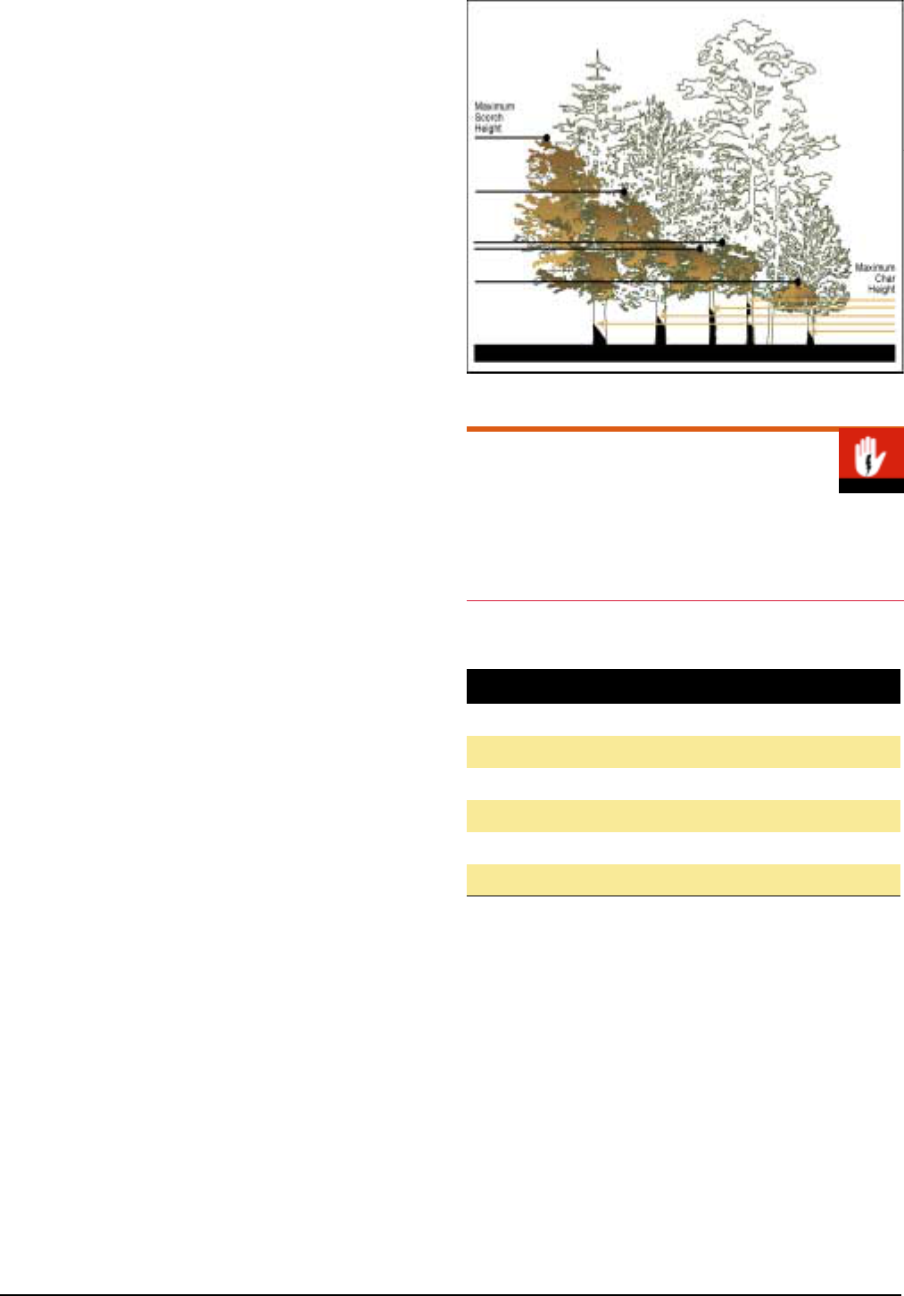
Scorch Height

Record the tree tag number (Tag), whether the tree is

alive (L), dead (D), resprouting (R), consumed/down

(C), broken below BH (B) or cut stump (S) (Live

Code), maximum scorch height (ScHgt), and the

scorched proportion of the crown (ScPer). See Glos-

sary for definitions. Trees that have fallen should be

noted, though they will be recorded during the year-1

remeasurement. You may also record char height

(Char), an optional variable, on FMH-20.

Estimate the maximum scorch height on each over-

story tree two weeks to two months after the fire has

burned across the monitoring plot. Note: If another

time frame (e.g., 3 months or year-1 postburn) exposes

scorch patterns more definitively, measure scorch

height again at that time and enter the data with the

other Post data. Record this information in the Notes

section of the FMH-4.

Maximum scorch height is measured from ground

level to the highest point in the crown where foliar

death is evident (see Figure 35). Some trees will show

no signs of scorch, but the surrounding fuels and vege-

tation will have obviously burned. In this case, you can

estimate scorch height by examining adjacent vegeta-

tion. It may be useful to produce a graph of scorch

heights to show the variation around the average. Man-

agers may want to correlate scorch height with the pre-

burn locations of large dead and down fuels; these

correlations usually require photographs or maps of

fuel pockets.

Percent Crown Scorched

For each overstory tree, estimate the percent of the

entire crown that is scorched. Average percent crown

scorched may be calculated, but percent crown

scorched is a better indicator of individual tree mortal-

ity.

OPTIONAL MONITORING PROCEDURES

Char Height

You can often measure char height simultaneously

with scorch height. To obtain an average maximum

char height, measure the height of the maximum point

of char for each overstory tree (see Figure 35). For

these data calculate the mean of maximum char

heights. It may be useful to note on the data sheet the

extent of the cambial damage to the tree and to

describe the char on the ground surrounding each tree

in the Notes section of FMH-20.

Figure 35. Scorch and char height.

Scorch and Char for Pole-size Trees

(Optional)

You may collect scorch height, percent crown scorch,

and char height for pole-size trees if these data are

important to resource and/or fire management staff.

Table 29. Accuracy standards for during burn and

immediate postburn (RS) variables.

Fire Behavior and Severity

Flame Length or Depth/ROS <10 ft ± 1 ft

>10 ft ± 5 ft

Burn Severity ± 1 Class

Scorch/Char Height <10 m ± 1 m

>10 m ± 5 m

Percent Crown Scorch ± 10%

Chapter 5 n Vegetation Monitoring Protocols 111

File Maintenance & Data Storage

PLOT TRACKING

One of the most important aspects of managing a

monitoring program is having a system for tracking the

number of plots. One of the most concise methods is

to create a Master plot list. Within this list all plot

name changes, burn unit locations, burn dates, and

Table 30. Example system for tracking plots.

sampling dates are contained within a single document;

an example is included below (Table 30). This type of

document can easily be created in a spreadsheet pro-

gram such as Microsoft Excel. Maintain a master list

for all plots. It is the responsibility of the lead monitor

to maintain this list.

Former Plot

Name & #

Current Plot

Name & #

Burn

Unit

Burn

Date(s)

Pre 01Post 01yr01 01yr02 02Post Notes

BSAME3T0401 BADSPD0401 Green 10/93 08/90 11/93 08/94 08/95 Tags not

Meadow changed

FQUGA4D0921 Coyote 8/92 7/92 10/92 7/93 8/94 10/97 Did not actually

Creek 9/97 burn in ‘97

MONITORING TYPE FOLDERS

For each monitoring type, create a folder to hold all

information pertinent to that monitoring type. At min-

imum each folder should contain the following:

• Monitoring type description sheet

• Master list of all plots within the monitoring type

• Master map(s) with all plots within monitoring

type marked

• Minimum plot calculations by monitoring type

• Any burn summaries for burns conducted within

the monitoring type

• All data analyses for the monitoring type

MONITORING PLOT FOLDERS

Establish a raw data file for each monitoring plot.

Within the file, store all data sheets and maps for that

plot, including the Plot location data sheet (FMH-5).

File data sheets in numerical order by data sheet num-

ber. All plot folders should then be filed by monitoring

type. In some parks, plot folders may be filed by burn

unit. If this is the case, all plots should be filed alpha-

betically by monitoring type and then in numerical

order by plot number within each monitoring type.

SLIDE—PHOTO STORAGE

To protect your originals, make a duplicate set of slides

for use in the field. High temperatures and exposure to

sunlight, ash, and dirt reduce the lifetime of a slide.

Offsite Data Backup

It is strongly recommended that you store backup digi-

tal or hard copies of all FMH-5 (Plot location data

sheets), including the maps illustrating the directions to

the plots, with your regional coordinator or in another

off-site location. Offsite storage of your data is the only

way to protect it in the event your office is burglarized

or hit by fire or flood. In the event an original map is

lost or destroyed, you will have a copy with which to

relocate the plot. Remember: a lost plot is lost data.

Place all slides or photos in archival quality slide or

photo holders, which in turn should be stored in archi-

val quality binders or a slide file. Store slides in a cool,

dry environment away from sunlight. Though it limits

ease of access, the optimum storage area is with the

archive division of your park. If you have access to a

high quality scanner, you may want to scan the slides

so that you have digital backups (this will also allow

you to print copies to take with you to the plot).

File all photographic materials by monitoring type and

then numerically by plot number. File slides for each

plot photo (e.g., 0P–30P) sequentially by sample visit:

00 PRE, 01 Burn, 01 Post, 01 yr01, 01 yr02, 01 yr05, 02

Burn, etc.

FIELD PACKETS

Create field packets to carry copies of monitoring data

for field reference. Keep these packets in sturdy fold-

Fire Monitoring Handbook 112

ers. Your field packets should include the following

items for each plot:

• Set of print copies of the preburn photos

• Copy of all maps

• Copy of the FMH-4 (Monitoring type description

sheet)

• Copy of the FMH-5 (Plot location data sheet)

• Copy of the park’s FMH-6 (Species code list)

• Copy of the data from the most recent visit, so that

you can consult species codes, check tree diameters,

verify protocols, etc.

• Log of problems encountered on the plot, plot name

changes, species to be verified, etc. (see Plot mainte-

nance log, FMH-

25)

DATA PROCESSING AND STORAGE

The current National Park Service protocol is to enter

all data into the FMH.EXE software (Sydoriak 2001).

Data entry screens are designed to mimic the standard

data sheets. The addition of pull-down menus, specific

help, and extensive error-checking makes FMH.EXE

powerful and easy for computer novices to use. Any

software that can access xBase files (including

Approach, dBASE, Visual FoxPro (or FoxBase), and

Paradox) can be used to edit, enter and analyze FMH

data, but using FMH.EXE will enhance data integrity

by providing validated data entry; in addition, it auto-

mates standard data analyses.

Use the Quality control checklist (FMH-24) whenever

you enter and quality check your data. Record the date,

your initials, and the computer you used. If you find

any problems while you are entering data, use the Plot

maintenance log (FMH-25) to describe the problem

and what you did to correct the problem. Keeping logs

such as these serves as a valuable record of data collec-

tion and entry problems.

Data Backup

As is recommended with all computer work, backup

often, particularly after a large data entry session. The

FMH software automates data backup onto a floppy

diskette. For very large databases the FMH software

can zip (compress) your database(s) so that all data can

be contained on a single floppy diskette. It is also

important to send copies of your database to your

regional coordinator annually (at a minimum) for

safe storage.

Chapter 5 n Vegetation Monitoring Protocols 113

3

Ensuring Data Quality

The data you have so painstakingly collected are going

to be analyzed, and management decisions will be

based on these analyses. One or two errors per data

sheet can add up to a significant error, which if not

detected can lead to erroneous conclusions about

observed changes.

Standards for high data quality begin with accurate

field data collection and continue in the office with

accurate data entry into the FMH software. Ensure

high data quality standards by properly training field

staff, and developing a system of data quality checks

both in the field and in the office.

Proper training of field staff may involve setting up a

practice plot on which each member of the staff has an

opportunity to measure and remeasure each of the

variables sampled. Comparison of the values will reveal

those sampling variables where there can be a high

degree of variation in the values obtained. Discuss the

variations in values with staff members and clarify

proper sampling techniques. Use the accuracy stan-

dards at the end of each section in this chapter as a

guideline for how close your measurements need to be.

Example:

Litter and duff depth measurements often have the

highest degree of error due to the difficulty of identi-

fying the difference between these two layers. Ask

each member of the field staff to measure litter and

duff at a series of sample points. Compare the results

and discuss the definition of litter and duff and how

to identify the two layers. Have staff members sample

several more points until each staff member’s mea-

surements are within 0.5 in of each other.

QUALITY CHECKS WHEN REMEASURING

PLOTS

When remeasuring a plot it is important to review the

previous year’s data. Refer to the Plot maintenance log

(FMH-25) to see if there are any problems that need to

be corrected. Use the previous year’s data sheets as

templates for gathering the subsequent data. It is

essential that significant changes seen year to year be

true changes and not the result of omission or errors

in data collection.

Monitoring Type

Ensure that previous monitors had a clear understand-

ing of all aspects of the monitoring type description.

Has the description changed since the plot was

installed? Were the plots established randomly? Did

earlier monitors use different sampling areas or meth-

ods from one plot to the next? Are these methods dif-

ferent from the methods you currently use? See

“Monitoring Type Quality Control” on page 51 for

further reference.

Plot Location Data

Were you able to relocate the plot based on the direc-

tions on the FMH-5? Were the directions clear? Was

the map easy to follow? Did you find all of the ele-

ments of the written directions clearly illustrated on

the hand-drawn map?

Some of the important variables to compare year to

year are as follows:

Photo Documentation

Use the previous year’s slides (or prints) to take plot

photos with the same field of view year to year. Take

time to align tree limbs, ridgelines or rock outcrops in

the same position as seen in the previous year’s photo

so that changes in vegetation over time in relation to

these features can be seen year to year.

Herbaceous Cover

Generate a data summary for each plot using the FMH

software. Review this summary prior to reading the

herbaceous transect, so that you will know what spe-

cies you may encounter. When you finish reading the

transect, check off all the species you encountered on

the data summary from the previous year. Look for

any species not checked off the list.

Shrub Density

In some instances individual root crowns can be

obscured by grass and other herbaceous plants. Use

the previous year’s data as a guide to how many indi-

viduals were counted within each interval of the brush

belt.

Overstory and Pole-size Trees

Use the previous DBH measurement as a guide to

ensure that you are making the current measurement at

the same point as the previous measurement. Watch

Fire Monitoring Handbook 114

for large variations in DBH from one year to the next.

Confirm that trees marked dead at immediate post are

still dead at year-1. If they are not, correct the data for

the immediate postburn visit on both the hard copy

and in the database. Check each tree along the sam-

pling area perimeter to ensure that >50% of the base

of the tree is within the sampling area. Also, check to

see if crown or damage codes are fluctuating from one

year to the next.

Downed Fuel Load

Check your data against realistic expectations. The

number of 100-hr and 1000-hr logs do not generally

fluctuate within a year’s time. Rotten 1,000-hr logs do

not generally increase in number immediate postburn.

100-hr logs may be consumed immediate postburn

(1,000-hr logs rarely are), but between year-1 and year-

2 these logs should still be present. Make sure you also

check for fluctuations in slope measurement for each

fuel transect.

QUALITY CHECKS IN THE FIELD

Budget a little extra time at the completion of a plot in

order to save a repeat trip to a plot to collect data that

were overlooked. Before leaving the field, perform the

following checks:

Monitoring Type

Make notes on the quality of the monitoring type

description, as your feedback is critical to the authors

of that description. Is the description clear to all mem-

bers of the crew? Does the description contain enough

quantitative and qualitative information for your crew

to make the decision to accept, or reject a plot? Do the

sampling areas seem too large or too small? Do the

sampling protocols seem appropriate? Is it clear why

managers have asked you to collect data for optional

variables? See page 51 for further reference.

Data Sheets

Are they complete? Is any information missing? For

example, has live-dead been indicated on all tree data?

Are all species codes identifiable and correct?

Vouchers

Have voucher specimens been collected for

unknowns? If a specimen could not be collected, has

the unknown been adequately described, drawn or

photographed? Is this information sufficient to distin-

guish among unknowns? Are collection bags clearly

labeled with plot I.D., date and contents? Use the

voucher labels on the back of the FMH-6.

The FMH-6 serves as a list of each unknown you

encounter in order to help monitors quickly identify

which plants need to be collected. Carry this list from

plot to plot to ensure that you use the same code until

the plant is collected and identified.

Mapping

Have monitors taken azimuths and distances to and

from reference features? Have they drawn a rough

map showing the plot location in relation to other

prominent features? It is often difficult to recreate the

spatial arrangement of features from memory in the

office.

Accurate Maps

Accurate mapping of plot locations is one of the most

important tasks monitors have to complete. Too often

mapping is done hurriedly at the completion of a plot.

Allow yourself ample time to take accurate azimuths,

measure distances, and write a clear description of how

to get to the plot. A plot that cannot be relocated is

data lost.

QUALITY CHECKS IN THE OFFICE

If necessary, make a more thorough check of the data

sheets when reaching the office. Check your data

sheets as soon as possible after you sample the

plot. Your mind will be fresh, and you can clearly elab-

orate upon your cryptic notes.

If you cannot identify unknowns within a day or two,

press the voucher specimens. Monitors often leave

specimens in collection bags for too long and they

become moldy and unusable. Keep a running log of

voucher specimens collected. Store vouchers properly

so they can be used at a future date (see Appendix C

for guidelines).

Have a central filing area where you can store original

data sheets (organize by task, e.g., to be checked for

quality, to be entered, needs discussion, to be filed)

until they are filed. Organize the data sheets in a logical

order, e.g., alphabetically by monitoring type, then

numerically by plot number, then numerically by data

sheet number. Use the Quality control checklist

(FMH-24) to ensure that all data and supplemental

information have been collected, entered, and quality

checked for a particular plot.

Chapter 5 n Vegetation Monitoring Protocols 115

QUALITY CHECKS FOR DATA ENTRY

For even the most accurate typist, it is imperative that

you check each data sheet entered into the FMH soft-

ware. Although the FMH software has extensive data-

checking capabilities, it cannot detect typographical

errors such as entering a DBH of 119.0 instead of 19.0.

Once you have entered the data from a data sheet,

compare the data on each data sheet with the database,

and check those data line by line for accuracy. Gener-

ally, it is better that an individual other than the person

who entered the data check the data sheet.

When entering data, record any problems on the Plot

maintenance log (FMH-25). Make sure that you

resolve each problem and then check it off the log.

The FMH software has a data-checking mechanism for

each data sheet. You should use this to check each data

sheet after you enter it (optionally, you can check all

data sheets at a single time). Make sure that you have

error-checked each data sheet before you conduct any

data analyses.

Finding Errors in Density Data

Trees, shrubs, or herbs are occasionally missed, or erro-

neously called dead one year, then found to be alive the

next. If you have collected data on your plots for two

or three years, one technique for finding these errors is

to use the analysis option in the FMH software (multi-

ple burn status graphics), on a single plot basis. Per-

form this analysis for all visits to a single plot, by

choosing the “select plot” option within the analysis

menu. Look at the graphical or numerical representa-

tion of the data and check for any fluctuations in den-

sity that might not be accounted for by death or

recruitment, or the absence of change where change is

expected.

Finding Errors in Species Cover Data

Shrubs or herbs are occasionally missed, or errone-

ously called one species name one year and another the

next. If you have collected data on your plots for two

or three years, use the technique described in the

“Finding Errors in Density Data” tip box. Look at the

graphical or numerical representation of the data and

check for any fluctuations in species within genera or

with species that are often mistaken with each other,

which might not be accounted for by death or recruit-

ment, or the absence of change where change is

expected.

Finding Errors in Fuels Data

Larger diameter size class (>1”) fuels are occasionally

missed or placed in the wrong class, or 1,000-hr logs

are erroneously called rotten one year and found to be

sound the next. Monitoring crews can have varying

understandings of the difference between litter and

duff from one year to the next. If you have collected

data on your plots for two or three years, use the tech-

nique described in the “Finding Errors in Density

Data” tip box. Look at the graphical or numerical rep-

resentation of the data and check for any fluctuations

in fuel load, within each category of fuel, which might

not be accounted for by decomposition or combustion,

or look for the absence of change where change is

expected.

Data Management

For an in-depth discussion of data management, con-

sult the data management protocols used by the NPS

Inventory and Monitoring Program (Tessler and Greg-

son 1997).

Fire Monitoring Handbook 116

Clean Data

If you follow all of these quality control guidelines,

your data generally should have the following charac-

teristics:

• No data are missing from either the data sheets or

from FMH.EXE

• No transcription errors exist, i.e., the data sheets match

the FMH.EXE screens perfectly

• The data have been error-checked by the software and

by an experienced field person

• Data from different visits are at the same level of qual-

ity

Plot visits conducted by different field staff or at differ-

ent times are especially prone to data errors—be sure

to confirm species identification and naming consis-

tency, check for fluctuation of individuals between

classes (e.g., live and dead, height, crown, age) and

ensure that data follow a logical order (e.g., individuals

should not decrease in diameter, damage, or maturity).

Chapter 5 n Vegetation Monitoring Protocols 117

Fire Monitoring Handbook 118

Data Analysis and Evaluation

6

Data Analysis & Evaluation

“Take nothing on its looks; take everything on evidence. There’s no better rule.”

—

Charles Dickens

Analyzing fire monitoring data and using the results to

evaluate the prescribed fire management program are

the keys to successful adaptive management. The

results of a monitoring program are used primarily to

determine whether management objectives are being

met. The results can verify that the program is on

track, or conversely, provide clues as to what may not

be working correctly.

Completing the process of data analysis and program

evaluation is critical, because the role of monitoring is

to gather information to guide the management pro-

gram. The main purpose of this handbook is to pro-

vide valuable feedback for management; if this

information is not used as a feedback tool, then the

monitoring program will not have served its purpose.

Without proper analysis, the monitoring data may at

best be useless to managers, and at worst provide mis-

leading information.

The success of a fire monitoring program is strongly

dependent on the fulfillment of clearly defined respon-

sibilities at all stages, including analysis and evaluation.

The specific duties of management staff have been

reviewed in Chapter 1 (page 4). Because the analysis

and evaluation process is complex and critical to the

monitoring program, the procedures outlined in this

chapter should be performed or closely supervised by

staff with background and experience in scientific

analysis.

The steps involved in data analysis and program evalu-

ation include:

• Document the analysis process

• Examine and quality-check the raw data

• Summarize the monitoring data

• Evaluate whether management objectives were met

• Adjust the fire monitoring program or management

actions (if needed)

• Disseminate the results

• Review the monitoring program periodically

Prescribed fire program evaluation is the process by

which monitoring becomes more than an exercise in

data collection. It requires the coordinated efforts of

fire management, resource management, and research

expertise. At levels 1 and 2, the data are needed to

guide decisions for ongoing fires. At levels 3 and 4,

careful and prompt evaluation of short-term and long-

term change data will provide information necessary

to support and guide the prescribed fire management

program by determining whether the program objec-

tives are being met.

LEVEL 3: SHORT-TERM CHANGE

Summarizing data to assess short-term change (see

page 5) involves analysis of the variables specified by

short-term change objectives. These objective vari-

ables were selected as the attributes measured to evalu-

ate the management objectives. When you summarize

short-term data you are essentially comparing the pre-

burn and specified postburn conditions to evaluate the

achievement of short-term objectives. In addition to

summarizing data for each objective variable, you

should also analyze all other measured variables to

detect changes and identify any unexpected short-term

results.

Example:

A short-term change objective in the sand pine scrub

monitoring type is to reduce mean shrub cover to

30–50% one year postburn. In this case, the one year

postburn shrub cover data would be analyzed for all

the plots in the sand pine scrub monitoring type to

determine whether the mean falls within the 30–50%

range. Trend analysis from other measured variables

can be examined for desirable or undesirable trends,

e.g., an increase in the mean non-native species cover

in the understory.

LEVEL 4: LONG-TERM CHANGE

Evaluating the prescribed fire program’s long-term

success is difficult because long-term change (see page

5) objectives often do not exist, or if they do exist, they

119

often are not specific or measurable. Yet the long-term

outcome is the basis for measuring the attainment of

broad goals and the success of a prescribed fire man-

agement program. For example, where the long-term

goal is to restore the natural conditions and processes

to an area, knowing that the program met a fuel reduc-

tion objective two years postburn is meaningless if the

area is never burned again and eventually reverts back

to unnaturally heavy fuel load conditions.

Monitoring long-term change is essential for detecting

undesired effects of management activities. Therefore,

the data analysis, interpretation, and response associ-

ated with long-term change requires special attention.

Although monitoring plots are designed to quantify

the extent of change from preburn conditions, the

complex interaction of ecological processes (including

fire, succession, herbivory, competition, disease, and

climate change) makes the results of long-term change

difficult to interpret. In assessing long-term change,

data from unburned plots outside this monitoring sys-

tem, e.g., inventory and monitoring plots, can be espe-

cially useful.

Example:

A long-term change objective in the mixed-grass

prairie monitoring type is to increase the mean native

species percent cover by at least 20% after three pre-

scribed fire treatments occurring every 3–8 years.

Here, the postburn percent cover data would be ana-

lyzed for all the plots in the mixed-grass prairie mon-

itoring type after they were burned three times to

determine whether the mean native species percent

cover had increased by at least 20%.

Due to the complex nature of non-native species

invasion in which many factors may be involved,

information on native/non-native species percent

cover in similar areas that have not been burned

would be useful for comparison, especially if the

objective was not met.

Sound management judgment, based on broad review

and in-depth knowledge of local ecology, is essential

for identifying long-term trends. Trends may be easy to

recognize (influx of non-native plants, high mortality

of one species) or complex and subtle (changes in

stand structure, altered wildlife habitat, or insect or dis-

ease infestations). It is essential that managers remain

familiar with the character of the monitoring type

throughout its range in order to maintain sufficient

breadth of context for interpretation of long-term

trends. Joint review of long-term data by fire, research,

and resource personnel will help identify and define

trends.

Fire Monitoring Handbook 120

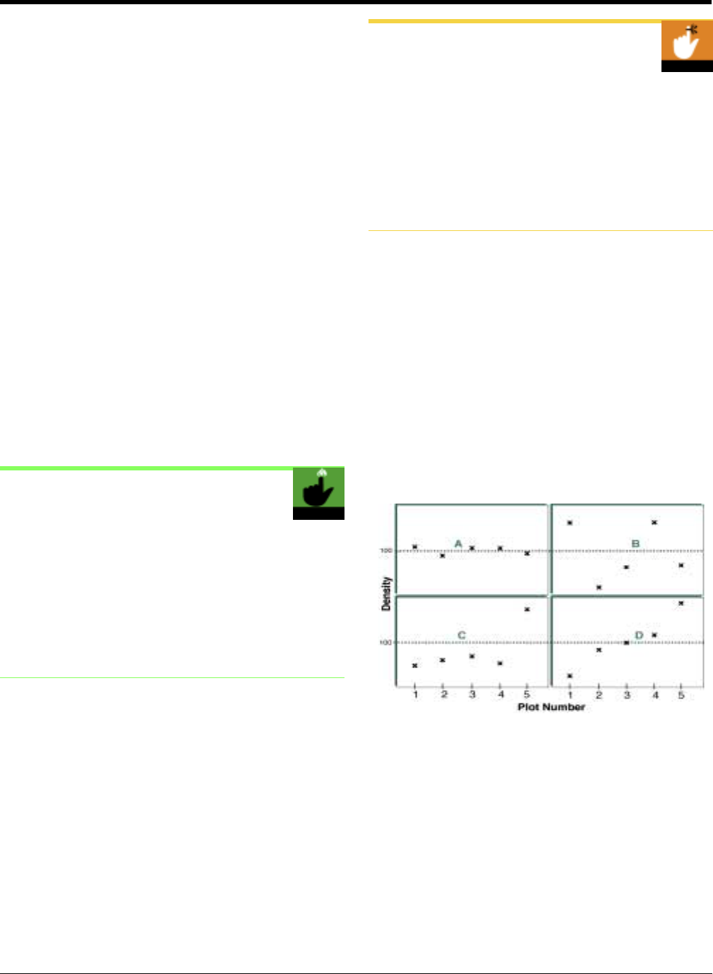
The Analysis Process

DOCUMENTATION

The analysis process can be complex; therefore, docu-

menting the steps in the process is important so that

the reasoning behind the decisions made along the way

is clear. Documentation should be clear and thorough

enough so that someone else can repeat the process

used to obtain results, and verify or refine the interpre-

tation of those results. The long-term data will be used

for many years. In the future, someone will need to

understand how the monitoring results were obtained

and how decisions were made based on those results.

Data Analysis Record (FMH-26)

A form to document the analysis process has been

designed to complement the fire monitoring program

and provide a link between the management objec-

tives, the raw data, and the results. The Data analysis

record (FMH-26) has space for a discussion of the out-

puts relative to the management and monitoring objec-

tives. This form will help document the analysis

process so that the results can be verified and repeated

if necessary.

Data Analysis Record

• Store the Data analysis record (FMH-26) together

with all graphs and analysis output sheets and the

Monitoring type description sheet (FMH-4).

• Document program changes directly on the Data

analysis record or in another format and store in a

clearly labeled binder that is easily accessible to man-

agers.

Program Changes

In addition to documenting the analysis process, you

should document any resulting modifications that were

made to the monitoring or management program.

These modifications may include changes to monitor-

ing protocols, burn prescriptions, treatment strategies,

or objectives.

Program Changes

The historical record of any program changes is critical

for understanding the evolution of knowledge and

management actions over time. This documentation

may be needed at some point in the future to demon-

strate that the course of the management program fol-

lowed a logical progression validated by the monitoring

data.

EXAMINING THE RAW DATA

Before you summarize the data, you will find it helpful

to examine the data for each individual plot. Graphs of

the objective variable values for each plot can reveal

patterns that are not apparent from descriptive statis-

tics such as the mean and the standard deviation. For

example, Figure 36 shows four samples each with a

sample size of five plots, and each with a mean of 100.

Without a graph of the data, one might assume from

the means that the data from the four samples were

identical.

Figure 36. Four samples each with a sample size of five

plots, and each with a mean of 100.

Graphically displaying the values for each plot is one

way to check data quality. Extreme plot values that

might not be apparent from the mean value may be

obvious from the graphic display of each plot’s values.

If you find an extreme value, check the database and

raw data sheets for errors.

In addition, some types of inferential statistical tests

assume that the data are normally distributed, in what

is often referred to as the standard normal distribution

Chapter 6 n

nn

n Data Analysis and Evaluation 121

or ‘bell-shaped’ curve. A graph of the individual plot

data will show whether this assumption has been met

or whether the data distribution is skewed. For further

information regarding the standard normal distribu-

tion, see any statistics text (e.g., Norman and Streiner

1997, Zar 1996).

SUMMARIZING THE DATA

After all plots within a monitoring type burn, and data

have been collected for the entire sample, summarize

the results so that they can be interpreted. To summa-

rize the data, you can use descriptive statistics to

reduce many observations (many plot values) to a sin-

gle number that describes the sample as a whole. The

sample mean is a frequently used statistic that

describes the central tendency of the sample, or the

average of all plot values for a variable. The sample

mean is used as an estimate of the population mean. If

the data are not distributed normally, consider using

other measures of central tendency, e.g., the median or

the mode (see any statistics text for definitions). It is

customary to report the sample mean along with some

measure of variability.

Reporting Data Variability

Since the sample mean is only an estimate of the true

population mean, reporting the sample mean values

without saying something about how good the esti-

mate is likely to be is inappropriate (the danger is that

people may assume that the sample mean is the popu-

lation mean, when it is really only an estimate).

As stated above in the section on examining raw data,

displaying all the individual plot data in a graph is use-

ful to visually depict the differences among plots. You

should also use one of several measures, either the

standard deviation, standard error, or confidence inter-

vals, to numerically report the variability in the

results.

Standard deviation—variability in the data col-

lected

To report the variability among plot values in the sam-

ple, calculate the standard deviation. This measures

how well the average value describes individual obser-

vations in the sample. This measure of variability, or

dispersion, will tell you whether the observations are

very close to the mean or whether many of them are

quite different (Figure 37).

Figure 37. Standard deviation is generally an average of

the lengths of all the arrows (distances from the sample

mean).

Standard deviation is a measure of the distribution

(spread) of observations (plot values) in a sample from

the sample mean. It is the variability of the data

expressed by taking the square root of the variance

(which is the sum of squares of the deviations from the

mean). If the data are distributed normally (have a

shape like the normal distribution), then approximately

68% of the observations will fall within one standard

deviation of the sample mean and approximately 95%

of the observations will fall within two standard devia-

tions of the sample mean.

A large standard deviation value (high variability) could

indicate an error in the data (see page 131), or that the

data are truly highly variable. Highly variable data

could have one or more implications: more plots may

need to be installed, the method used to collect the

data may not be the most appropriate, and/or the vari-

able measured is patchy across the area sampled.

To calculate the standard deviation, you need the fol-

lowing inputs:

• Values for each observation (plot)

• Mean of the sample (mean of plot values)

• Number of plots in the sample

The FMH software calculates standard deviation. For

the formula to calculate the standard deviation, see

page 216 in Appendix D.

Fire Monitoring Handbook 122

Example:

Three monitoring plots located within a particular

burn unit have preburn 1,000-hr fuel loads of 18.5,

4.2, and 6.7 kg/m

2

respectively. Therefore, the mean

± one standard deviation is 9.8 ± 7.6 kg/m

2

. The

summary results are not used to make generalizations

to the burn unit or monitoring type as a whole, but

simply to show what the mean and variability is for

the 1,000-hr fuels in the three plots. The standard

deviation of 7.6 indicates that the variability in 1,000-

hr fuel load among the three plots is high (almost

equal to the mean of 9.8). In this example, the indi-

vidual plot values are very different from each other

and vary greatly from the mean value of 9.8 kg/m

2

.

Standard error—precision of the mean

Although in the design of the monitoring program the

scientific method is used to obtain a random sample,

any particular sample (collection of plots in a monitor-

ing type) is just one of many possible samples. One

random sample of 10 plots would likely give different

results than another random sample of 10 plots; addi-

tionally, a sample of three plots would have different

results than a sample of 300 plots. Standard error is a

measure of the variability related to the fact that only a

portion of the entire population is sampled.

If many different samples were taken, each consisting

of the same number of plots, the standard error is a

measure of how close the sample means are likely to be

to the true population mean, or what is known as the

‘precision of the mean.’ Standard error is the variability

of the theoretical distribution of the sample means

for a given sample size. The shape of the distribution

of possible sample means changes depending on sam-

ple size. The larger the sample size, the closer the sam-

ple mean is likely to be to the true population mean;

therefore, standard error is directly related to sample

size (see Figure 38).

Based on these theoretical distributions of sample

means, if many samples of the same size were taken,

then approximately 68% of the sample means would

fall within one standard error of the true population

mean, and approximately 95% of the sample means

would fall within two standard errors of the true popu-

lation mean.

Figure 38. Three sampling distributions (of different

sample sizes) with the same mean.

This figure illustrates how standard error decreases as sample

size increases.

To calculate the standard error, you need the following

inputs:

• Standard deviation of the sample

• Number of plots in the sample

The standard error is the default measure of variability

calculated by the FMH software. See page 218 in

Appendix D for the formula to calculate the standard

error.

Example:

In the tallgrass prairie, 12 monitoring plots were

established. The native perennial grass mean relative

cover ± one standard error is 48.8 ± 3.4%. This stan-

dard error means that if many samples of 12 plots

were taken, approximately 68% of the sample means

would fall within ± 3.4% of the true population mean

for relative cover (and approximately 95% of the

sample means would fall within ± 6.8% of the true

population mean).

When to use standard deviation vs. standard error

Use standard deviation to report the variability of

the data itself—i.e., the variability among plots in the

sample.

Use standard error to express the precision of the

mean—i.e., the closeness with which the sample mean

estimates the true population mean.

Chapter 6 n

nn

n Data Analysis and Evaluation 123

The decision of which measure of variability to use is

not critical, as long as you report which one you are

using; standard deviation and standard error can be

derived from each other as long as you know one of

the two as well as the sample size.

Confidence intervals—precision of the mean with

stated level of confidence

While standard error is an estimate of the precision of

the sample mean, confidence intervals provide added

information about variability by using the standard

error along with a stated level of confidence. The con-

fidence interval is a range of values for a variable

which has a stated probability of including the true

population mean.

To calculate the confidence interval, you need the fol-

lowing inputs:

• Mean of the sample

•Standard error

• Desired confidence level (80, 90, or 95%)

• Critical value of the test statistic student’s t (two-

tailed), based on the selected confidence level (80,

90, or 95%) and the degrees of freedom (number of

plots - 1); the values used by the FMH software can

be found on page 220 in Appendix D

The FMH software calculates confidence intervals. For

the formula to calculate the confidence interval, see

page 219 in Appendix D.

Example:

Three plots show varying values for seedling tree

density: 120, 360, and 270 seedlings/ha, with a stan-

dard error of 70. The confidence interval is expressed

as a range and probability; therefore, there is an 80%

probability that the true population mean value for

seedling tree density is between 118 and 382 seed-

lings/ha. Alternatively, you could state that the 80%

confidence interval is 250 ± 132 seedlings/ha.

Summarizing Results

When summarizing results, always report the mean

with some measure of variability (either standard devia-

tion, standard error, or confidence interval), state

which measure of variability was used, and be sure to

include the sample size (number of plots).

RECALCULATING THE MINIMUM SAMPLE

SIZE

Once all of the plots in a monitoring type have burned

and monitoring has been conducted throughout the

postburn time period of interest (as determined by

your objectives), recalculate the minimum sample size

needed. Determining the number of plots needed to

achieve the desired certainty in the specified postburn

results should be done in one of two ways, depending

on the type of management objective: change (see page

25) or condition (see page 26).

To assess, as early as possible, whether more plots will

be needed, you can perform this calculation after some

of the plots (3–5) have reached the postburn time

interval rather than waiting for all plots to reach the

time interval.

Condition Objectives

To determine whether you have installed the number

of plots sufficient to assess the postburn target or

threshold objective, you should recalculate the mini-

mum sample size after the plots have burned and

reached the appropriate postburn time interval (as

determined by your management objectives). Use the

same formula (see page 216, Appendix D) used for the

preburn plots (see page 49 for discussion) to deter-

mine the appropriate number of plots needed. Your

chosen confidence and precision levels should remain

the same as they were in the initial minimum sample

size calculation unless your monitoring objectives have

changed for some reason.

If the variability in the postburn data is about the same

or lower than the preburn data variability, it is unlikely

that more plots will be needed. You may need to install

more plots if the postburn data variability is higher

than the preburn data variability.

Change Objectives

Once the appropriate number of plots have been

installed, burned, and measured at the postburn time

interval (specified by your management objectives), a

separate calculation will reveal whether you need to

install more plots to detect the desired amount of

change. For the formula to calculate the minimum

sample size for minimum detectable change (MDC)

desired, see page 217 in Appendix D.

If the variability in the differences between preburn

and postburn data is about the same or lower than the

preburn data variability, it is unlikely that more plots

Fire Monitoring Handbook 124

will be needed. You may need to install more plots if

the variability in the differences is higher than the pre-

burn data variability.

Minimum Sample Size for Minimum

Detectable Change (MDC)

This formula is a critical new addition to this hand-

book. For change objectives, calculate the minimum

sample size for the minimum detectable change you

desire before you fully evaluate whether you have met

your objectives.

For both condition and change objectives, if you

determine that more plots are needed after recalculat-

ing minimum sample size, install any necessary addi-

tional plots in areas of the monitoring type that have

not yet burned. If unburned areas no longer exist for

the monitoring type, then the current number of plots

must suffice and results should be presented with the

appropriate level of certainty.

Chapter 6 n

nn

n Data Analysis and Evaluation 125

Additional Statistical Concepts

In some cases you may want to perform additional sta-

tistical analyses. Several considerations may affect how

such analyses are performed, therefore, you should at

least be aware of how they might affect the monitoring

program results.

HYPOTHESIS TESTS

In addition to descriptive statistics (e.g., means and

measures of variability) and basic inferential statistics

(e.g., confidence intervals), hypothesis tests (also

known as significance tests) can be performed on

monitoring data. These tests are used to assess the

actual probability that the sample results were obtained

due to chance (as a result of random variation). The

concept of hypothesis testing is only briefly and gener-

ally discussed here. Examples of hypothesis tests

include analysis of variance (ANOVA), chi-square,

McNemar’s test, paired t-test, repeated measures

ANOVA, and Wilcoxin’s signed rank test. Review sta-

tistical texts (e.g., Norman and Streiner 1997, Zar

1996) for specific information on these tests.

A hypothesis is a proposed statement or theory that

provides a basis for investigation. A management

objective is like a hypothesis in that it makes a state-

ment that a particular condition or threshold is met, or

that some type of change from the current condition

occurred. This statement or objective is used as a basis

for comparing the data observed. A statement of no

difference is called the null hypothesis. In the fire mon-

itoring program, the null hypothesis is usually that a

condition or threshold was not met, or that no change

in a particular objective variable has occurred over a

preselected period of time.

A significance (hypothesis) test is “a procedure for

measuring the consistency of data with a null hypothe-

sis” (Cox 1977). The result of a hypothesis test is that

the null hypothesis is either rejected or not rejected. If

it is likely that the sample results occur reasonably

often in the population (based on estimates of variabil-

ity in the population), then there is no reason to reject

the null hypothesis. If only a small probability exists of

obtaining the sample results by chance, then the null

hypothesis is rejected. A one-sample hypothesis test is

one in which the results are compared with a hypothe-

sized value (e.g., comparing a postburn variable mean

with a desired mean value); a two-sample test is one in

which two sets of results are compared to determine if

there is a difference between them (e.g., comparing

preburn and postburn variable means).

In the context of monitoring, hypothesis tests assess

the probability that the results indicate a management

objective was met (as opposed to the results being due

to chance). If the hypothesis test concludes that the

observed mean, or change in the mean, of the variable

is not due to random variation, then the null hypothe-

sis is rejected in favor of an alternate hypothesis: the

mean value is different from the hypothesized condi-

tion or a change has occurred in the mean of the vari-

able.

Example:

The management objective in the ponderosa pine

forest monitoring type is to reduce live pole-size tree

density to less than 300 trees per hectare within two

years postburn. The null hypothesis is that the year-

2 postburn live pole-size tree density is greater than

or equal to 300 trees per hectare. A test to determine

whether the null hypothesis is rejected would be per-

formed.

or,

The management objective in the sagebrush steppe

monitoring type is to increase the mean percent cover

of native herbaceous species by at least 20% by 10

years postburn. The null hypothesis is that the year-

10 postburn mean percent cover of native herba-

ceous species is less than 20% greater than the preb-

urn percent cover, and a test to determine whether to

reject the null hypothesis could be performed.

Significance Level (α)

Because hypothesis tests assess the probability that

the results were obtained by chance, we need another

criterion to quantify the acceptable probability, thus to

indicate whether to reject the null hypothesis. This cri-

terion, called the level of significance, or α (alpha), is

the probability that an apparent difference occurred

simply due to random variability.

The significance level (α) must be determined before

the hypothesis test is performed; α is equal to one

minus the confidence level, which is chosen during the

design of the monitoring program before any data are

Fire Monitoring Handbook 126

collected (see page 27). For example, if the confidence

level chosen is 90%, then the significance level for a

hypothesis test is 10% (α = 0.10), and a probability of

obtaining the results due to chance less than 10%

would result in a rejection of the null hypothesis. It is

important to note that the significance level is not the

probability that the null hypothesis is true.

Two Ways To Be Wrong

With a hypothesis test, either of two clear conclusions

can result: 1) the test indicates that the results are not

likely to be due to chance (hence a real difference

exists or a real change has occurred), or 2) the test indi-

cates that the results are likely due to random variation

(thus a real difference does not exist or a real change

has not occurred). It is also possible that each of these

conclusions are either right or wrong (due to insuffi-

cient sample size, poor monitoring design, or inappro-

priate statistical tests). The combinations of all of these

possible conditions yield four potential outcomes of

hypothesis testing or monitoring for change. Two of

the possibilities are correct conclusions: 1) a condition

or threshold was not met or no change occurred and it

was not detected; and 2) a condition or threshold was

met or a real change occurred and it was detected

(Figure 39).

Two of the possibilities are incorrect conclusions or

errors: 1) a condition or threshold was not met or no

change occurred but the monitoring detected a change

or difference in condition; known as a Type I (or false-

change) error; and 2) a condition or threshold was met

or a real change occurred but it was not detected;

known as a Type II (or missed-change) error.

Null hypothesis is true:

A condition or threshold was not

met or no change occurred

Null hypothesis is false:

A condition or threshold was met or a

real change occurred

Null hypothesis rejected:

Monitoring detects a difference or

change

Type I Error

(false-change)

probability =

"

(significance level)

Correct

(no error)

probability = 1-

"

(confidence level)

Null hypothesis accepted:

Monitoring does not detect a difference

or change

Correct

(no error)

probability = 1-

$ (power)

Type II Error

(missed-change)

probability =

$

Figure 39. The four possible outcomes of hypothesis testing.

Type I error (false-change error)

Type I (false-change) error is comparable to a false

alarm. The monitoring program detects a difference in

condition or a change in an objective variable but the

difference or change that occurred was due to random

variability. This type of error can lead to the conclusion

that the management objectives were met using pre-

scribed fire, but in fact, the same the results could have

been obtained due to chance. Alternatively, an

unwanted change or difference might be detected (e.g.,

an increase in a non-native species) when no real

change took place, resulting in an unnecessary adjust-

ment to the prescribed fire program.

The probability of making this type of error is equal to

α (the significance level), which is equal to one minus

the confidence level chosen. For example, for a confi-

dence level of 80%, α is 20%, meaning that a false-

change error is likely to occur approximately 20% of

the time (or one in five times).

Type II error (missed-change error)

Type II (missed-change) error is analogous to an alarm

that is not sensitive enough. The monitoring program

does not detect a difference in condition or a change in

an objective variable, but in fact, a difference or a

change has taken place. This type of error may be criti-

cal, as it can mean that an unwanted decrease in a

favored species, or an unwanted increase in non-native

plants, goes undetected following prescribed fire appli-

cation. Alternatively, the management objective may

have been effectively achieved, but the results from the

monitoring program would not substantiate the suc-

cess.

The probability of making this type of error is equal to

β (beta), a value that is not often specified but that is

related to statistical power.

Power

Statistical power is the probability of rejecting the null

hypothesis when it is false and should be rejected. In

other words, power is the probability of detecting a

change when a real change (not due to random vari-

Chapter 6 n

nn

n Data Analysis and Evaluation 127

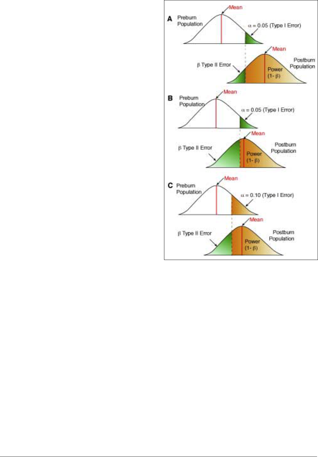
ability) has occurred. Power is equal to one minus

power (1-β)

—

the probability of making a missed-

change error. For example, if the power of the statisti-

cal test is 90%, then a missed-change error is likely to

occur 10% of the time. Conventionally, the minimum

level of power should be at least 80% (Cohen 1988), or

it should be equal to the confidence level (Peterman

1990).

Power is inversely proportional to the level of signifi-

cance for a given sample size. To simultaneously

increase power, or the probability of detecting a real

change (1-β) while decreasing the probability of com-

mitting a false-change error (α) you must either

increase the sample size or decrease the standard devi-

ation (see Figure 40). For change objectives, you

choose the level of power for calculating the minimum

sample size needed to detect the minimum amount of

change desired. Additionally, if you performed a

hypothesis test and it failed to reject the null hypothe-

sis, you can calculate power to determine the monitor-

ing program’s ability to detect a real change (and the

probability that a Type II (missed-change) error

occurred).

INTERPRETING RESULTS OF

HYPOTHESIS TESTS

After you have performed a hypothesis test you can

interpret the results by following a series of steps.

These steps are summarized in Figure 41. For results

that reject the null hypothesis, it is important to calcu-

late the power of the test to determine the monitoring

program’s ability to detect change. Once again, consult

a statistician for advice if you have any questions about

the statistical tests and interpretation of the results.

Pseudoreplication

Pseudoreplication is the use of inferential statistics to

test for treatment effects with data where treatments

are not replicated (though observations may be) or

replicates are not statistically independent (Hurlbert

1984). Pseudoreplication occurs, for example, when all

of the plots from a particular monitoring type are

located in one burn unit, and inferences about the

burn program in general (i.e., a treatment effect),

rather than the effects of one particular fire, were

made from the data.

Figure 40. Influence of significance and power for three

normally distributed populations.

A) A large difference in means between the preburn and

postburn population results in both a high level of power and a

low probability of Type I and Type II errors. This is ideal. B) A

smaller difference in means results in low power with a higher

probability of Type II error. C) Using a higher level of significance

substantially increases the power.

Ideally, plots would first be placed randomly across the

entire landscape and then treatments randomly

assigned to avoid the problem of pseudoreplication.

Within the constraints of a fire management program,

however, this type of design is usually not feasible. If

pseudoreplication is a serious problem in the sampling

design, and is not acknowledged, improper analyses or

data misinterpretation can result. See Irwin and

Stevens (1996) for a good overview of this often con-

fusing concept. Consult a statistician to determine if

pseudoreplication may affect the analysis of a particu-

lar monitoring program dataset.

Fire Monitoring Handbook 128

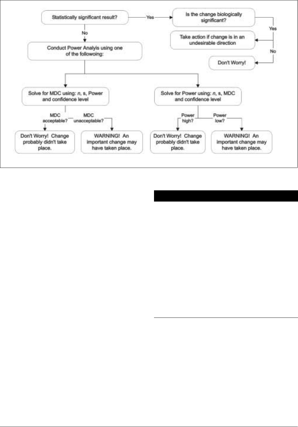
Figure 41. Steps in interpreting the results of a change over time statistical test.

Modified from Elzinga and others (1998).

Autocorrelation

All monitoring programs need to address autocorrela-

tion during the sampling design period. Data that are

autocorrelated are not independent over space or time

and therefore are more difficult to analyze. For

example, spatial autocorrelation can occur if plots are

placed so close together that the plots tend to record

similar information. In this situation, the data may

have an artificially low amount of variation. The fire

monitoring program addresses spatial autocorrelation

by using a restricted random sampling design to mini-

mize the chance that plots will be located in close

proximity to each other.

Temporal autocorrelation occurs when the same plots

are repeatedly measured over time, such as in the per-

manent plot methods used in this handbook. The data

from one year to the next are not completely indepen-

dent of the data in preceding years.

Example:

The preburn density of pole-size trees in one plot is

20 trees per hectare. Year-1 postburn, the pole-size

tree density is 5 trees per hectare, a decrease of 15

trees per hectare. The density two years postburn will

be limited by the fact that the year-1 postburn density

is now only 5 pole-size trees per hectare; a further

decline of 15 trees per hectare cannot occur. If the

same plot were not remeasured from one year to

next, the density would not be constrained by previ-

ous years’ values. The decrease that occurred

between preburn and year-1 postburn is likely to have

an influence on the amount of change in future years.

For this reason, special types of statistical tests are

designed for use in permanent plot situations.

Autocorrelated data require special procedures to per-

form statistical tests. Consult a statistician for assis-

tance in evaluating the extent of spatial and temporal

autocorrelation in the data and the appropriate statisti-

cal tests that may be needed.

Chapter 6 n

nn

n Data Analysis and Evaluation 129

The Evaluation Process

EVALUATING ACHIEVEMENT OF

MANAGEMENT OBJECTIVES

After all plots in a monitoring type (the sample) have

been installed, burned, and remeasured at the appro-

priate postburn time interval, use the results to assess

whether the management objectives were met using

the following steps:

• Compare the results with the target conditions or

desired change stated in the management objectives.

• Verify the results.

Comparing Results with Management Objectives

In order to determine whether the management objec-

tives were met, you must examine the monitoring

results for the variable and time period of interest, and

compare them to the objectives.

Condition objectives

If your objective specifies a postburn range of values,

or a threshold value, for a variable, calculate the post-

burn confidence interval and determine whether it

falls within the target range (or above or below the

threshold).

Example:

The management objective is to maintain a density

of live pole-size trees of 80–120 trees per hectare

within two years postburn. The monitoring objec-

tive specified an 80% level of confidence in the

results. The monitoring results indicate that the year-

2 postburn live pole-size tree mean density ± one

standard error is 92 ± 5 trees per hectare (n=14

plots). Calculating the 80% confidence interval indi-

cates that there is an 80% probability that the true

population mean falls between 85–99 trees per hect-

are. The objective was met (with 80% confidence)

because the confidence interval falls completely

within the target range of 80–120 trees per hectare.

If the confidence interval falls completely outside the

target range, or completely crosses the threshold value,

then you can be certain (with the chosen level of confi-

dence) that the objective was not met. If only part of

the confidence interval crosses the threshold, or falls

outside the target range, then you must be willing to

acknowledge that the objective may not have been met

because the true mean population value may fall out-

side the range desired (or may have crossed the thresh-

old), even if the mean value is within the target range.

Example:

Using the same management and monitoring objec-

tives as in the above example, you find that the year-2

postburn live pole-size mean density is 92 trees per

hectare, but the standard error is ± 10 trees per hect-

are (n=14 plots). The 80% confidence interval would

then be 78–106 trees per hectare. The objective was

met on the upper end of the range (less than 120

trees per hectare), but not on the lower end because

the true population mean may be between 78–80

trees per hectare. Even though the mean value of 92

falls within the target range of 80–120, in this case,

you must decide whether or not you can accept that

the true population mean may actually be 78–79 trees

per hectare.

The more the confidence interval falls outside the tar-

get range or falls above or below the threshold, the

greater the possibility that the true population mean

may not meet the objective condition. In order to nar-

row the confidence interval, you must either reduce

the variability in the data, increase the sample size, or

lower the confidence level (see page 27 for further dis-

cussion of this topic).

Change objectives

If a change from preburn conditions was specified in

the management objective, then you must compare the

preburn and postburn time interval results. Because

the same plots are being measured over time (perma-

nent plots), the pre- and postburn results are not inde-

pendent and must be treated differently than if they

were independent. You should therefore calculate the

difference between preburn and postburn values for

each plot and then calculate a mean of these differ-

ences. If the change is specified in terms of a percent-

age, you must calculate the percent change for each

plot and then calculate the mean percent change. You

can then calculate a confidence interval for the mean

of the differences or the mean percent change to see if

the confidence interval falls within the range of change

desired.

Fire Monitoring Handbook 130

Example:

The management objective is to reduce the mean

percent cover of live shrubs by 30–60% within one

year postburn. The monitoring objective specifies

that 80% confidence in detecting a 30% minimum

change was desired. The mean of the differences

between preburn and year-1 postburn mean live

shrub percent cover ± one standard error for 11

plots was 21 ± 4%. The 80% confidence interval is,

therefore, 15–27% cover. The objective was not

achieved because the amount of change (15–27%)

falls completely outside the target range of 30–60%.

If the confidence interval falls completely within the

target range specified in the objective, then the objec-

tive was met with that level of confidence. If only part

of the confidence interval falls inside the target range,

then you must be willing to acknowledge that the

objective may not have been met, because the true

mean population value may fall outside the range

desired even if the mean difference or mean percent

change falls within the target range.

Appropriate Statistical Tests

To determine the probability that the data suggest that

your objectives were achieved due to natural variability

in the data and not due to real change, you will need to

perform a statistical test appropriate for the type of

objective and data distribution. Seeking assistance with

these statistical analyses is highly recommended; the

tests and associated assumptions may be complicated.

Use caution—performing an inappropriate test

may cause managers to make misleading conclu-

sions about the results.

Verifying Results

Regardless of whether the objectives were met, be sure

that the results were not obtained due to errors at

some point during the process. To determine if faulty

results were obtained, take the following steps:

• Check for data entry or raw data errors (see pages

114–117)

• Verify that the burn or treatment prescription condi-

tions were met on all plots

• Ensure that the data analyses were run properly

• Look for extreme data values, which can contribute

to large standard deviations in the summary results

• Review the fire behavior observations for each plot

to check that the burn conditions were in prescrip-

tion

• Step through the analyses to be sure that the appro-

priate outputs were obtained

If obvious data errors do not exist, the prescription

conditions were met for all the plots, and the analyses

were run properly, then the results are likely to be

valid.

EVALUATING MONITORING PROGRAM OR

MANAGEMENT ACTIONS

Responding to Desired Results

If the results indicate that your management objectives

are being met, it is important to continue the monitor-

ing and burning schedule as planned to be sure that

further changes over time do not affect achievement

of objectives. If you gain any new knowledge about a

species or plant association, reevaluate the relevant

objectives to see if the program should be adjusted

based on the new information.

Although you may have achieved the current objec-

tives, you should be sure that your management objec-

tives consider the long-term outcome of repeated

treatments. After carrying out two or three more pre-

scribed burns in the monitoring type, will your objec-

tives remain the same, or will the long-term target/

threshold conditions change after the initial treatment?

Well-formulated long-term objectives will help the fire

management program progress in a timely, effective,

and ecologically sound manner.

Achieving the desired results—and meeting your man-

agement objectives—is no simple task. If you have

succeeded here, acknowledge the program accom-

plishment by sharing the results; it is important that

you advertise your success by informally recording the

results in a widely distributed report or by formally

publishing the results (see page 134).

Responding to Undesired Results

If your verified results indicate that management

objectives have not been met, take the following steps

to adjust the fire monitoring program or management

actions:

• Examine the monitoring program design

• Evaluate the treatment strategy

• Reassess the management objectives

• Seek special assistance from experts

Chapter 6 n

nn

n Data Analysis and Evaluation 131

Examining monitoring program design

Determine whether the monitoring program was

properly designed and implemented:

• Verify that the appropriate objective variables were

selected to assess the objectives.

• Check to be sure that the data were collected prop-

erly for the variables of interest.

Example:

If the objective was to increase the density of native

vs. non-native plants but only percent cover was mea-

sured, the data cannot indicate whether the objective

was met. Alternatively, if the transect was not long

enough to adequately measure percent cover of a

sparsely distributed plant species, then it would be

difficult to determine whether the objective for

increasing the species’ percent cover was met.

If you determine that a different objective variable is

needed or that the method used to measure an objec-

tive variable must be changed, you must install a new

set of plots for the monitoring type in areas that have

not burned. If all areas in the monitoring type have

already been burned, then you will not have the oppor-

tunity to attempt to assess objective achievement for

the initial prescribed burn. New plots could be

installed in the monitoring type, however, to determine

whether objectives are met by subsequent burn treat-

ments (repeat burns).

Evaluating treatment strategy

If the monitoring program design is valid, next deter-

mine whether the treatment strategy was adequate by

taking the following steps:

• Assess whether the treatment prescription is capable

of causing desired results.

• Decide whether the prescription parameters are

simultaneously attainable for all objectives.

• Assess whether a change in treatment strategy might

produce the desired results.

Tools are available for addressing some of these issues,

including developing burn prescriptions that are likely

to produce the desired effects. Some examples of pre-

dictive tools commonly in use today are RX WIN-

DOWS; BEHAVE; FOFEM; and FARSITE. It is

beyond the scope of this handbook to cover the use of

these tools; for additional information, talk to your

local or regional prescribed fire specialist.

You may be able to refine the treatment prescriptions

by comparing the prescriptions you used with success-

ful treatment programs (as described in the literature

or by other programs). For example, the majority of

the burn treatments may have occurred at the cooler

end of the prescription and the burn prescription may

be too wide at the cooler end. After you complete the

prescription verification process, adjust the treatment

prescription and start the monitoring type identifica-

tion, data collection and analysis process cycle over

again using the revised treatment prescription.

Inability to produce the desired results (meeting the

objectives) may be due to a number of other treatment

factors. After consulting with experts, carefully con-

sider which actions are most likely to yield the desired

results.

The treatment may be adjusted in a number of ways;

for example:

• Change ignition pattern, intensity of fire application,

or ignition technique (e.g., tandem torches vs. single

torch, or helitorch vs. drip torch).

• Switch treatment season. Use caution here. This

strategy can have dramatic consequences because of

the sensitivity to disturbance (fire or other distur-

bance, e.g., mechanical treatment) of plant and ani-

mal species at different phenological or reproductive

stages and because of large seasonal differences in

site moisture regimes.

• Change the frequency of treatments by reducing or

increasing the treatment intervals).

• Change the type or intensity of the treatment con-

ducted in conjunction with prescribed fire, e.g.,

switch from mowing to grazing, or change the mow-

ing height.

Treatment Prescription Modification

Modifying the treatment prescription, e.g., changing

the season of the burn, means that you must modify

your monitoring type. Remember that the monitoring

type is defined by the live vegetation and fuels present

as well as the treatment prescription. If either is altered,

you must create a new monitoring type to reflect the

changes.

Fire Monitoring Handbook 132

Reassessing management objectives

If the treatment strategy cannot be changed to achieve

the desired results, examine the objectives themselves

to:

• Decide whether the management objectives are

valid.

• Determine whether the management objectives are

achievable or whether conflicting objectives exist.

To determine the validity of an objective, make a realis-

tic assessment of the current and target conditions.

Decide whether the target conditions have ever existed

in the treatment area or whether some of the objec-

tives are unrealistic.

Example:

Increasing biomass productivity in a severely

depressed natural system, or restoring native grass-

lands where the seed source is no longer available or

the topsoil has been removed, may not be realistic

objectives.

Perhaps the objective is not reasonable given current

management constraints, or one objective may conflict

with achieving another objective.

Example:

A burn prescription calls for spring burns to maxi-

mize smoke dispersal. The primary ecological objec-

tive is to achieve a mean 30-70% mortality of the

pole-size trees within two years of treatment. It may

not be possible to generate the level of mortality

desired by burning in the spring. In this case, either

the burn season may need to be changed (if the mor-

tality objective is critical) or the mortality objective

needs to be reassessed (if smoke dispersal in the fall

would not be acceptable). Alternatively, methods

other than fire may need to be considered to achieve

the objectives given these and other constraints.

If an objective is not achievable, you have good reason

to refine the objective(s). Upon review and consulta-

tion with appropriate specialists, you may revise the

management objectives and you should then re-ana-

lyze the results to determine whether they meet the

revised objectives.

Seeking special assistance

Subject-matter specialist assistance is advisable when:

• Results are questionable

• Controversial issues arise

• Unanticipated changes occur

• A special investigation (research) is necessary

Prescribed fire programs are based upon the precept

that treatment by fire to meet management objectives

is generally defensible as a result of prior investiga-

tions. If the monitoring data suggest otherwise, the

foundation of the prescribed fire management pro-

gram is in question. The purpose of the monitoring

program is to recognize success and to discover and

learn from errors at the earliest point in time. If the

current management strategies are causing unexpected

and undesired results, it is important to suspend burn-

ing in the affected monitoring type until you can deter-

mine a different approach.

Example:

Winter prescribed burning was carried out to reduce

fuel and maintain the overstory for 20 years, without

monitoring, before a gradual and irreparable change

in the species composition and structure of the

understory was noticed (an increase in a noxious

non-native). If a monitoring program had been in

place, this type of change may have been detected

earlier and the burn prescription could have been

changed before irreparable harm had occurred.

Expert advice can help you thoroughly explore all pos-

sibilities and suggest reasons for the results. Document

any such exploration and the logic behind each reason.

Seek input from subject-matter experts, especially

those who understand fire or disturbance ecology,

have knowledge about the particular species or plant

association, and/or have knowledge about fire behav-

ior and effects. Places to find special assistance include:

• The Fire Effects Information System (FEIS) (USDA

Forest Service 2001)

• Other staff members, especially resource managers,

botanists, fire and/or plant ecologists

• USDA research and experiment stations

• USGS scientists

• Subject-matter experts from universities and the pri-

vate sector

• Library reference or Internet searches

If monitoring results are confusing or equivocal, initi-

ating a more specific research project may be the best

management alternative. When monitoring results sug-

gest a fundamental problem, follow-up research

projects must be initiated; these studies should be

Chapter 6 n

nn

n Data Analysis and Evaluation 133

designed by professionals and may take time to gener-

ate defensible and reliable results.

Undesired long-term change

As with undesired short-term results, management

response to undesired long-term change must be

based on informed projections and evaluation of

trends. You must determine whether the change will

affect untreated areas or shift balances in ways that

may threaten the integrity of the system. Most impor-

tantly, you must determine the ecosystem and manage-

ment trade-offs of ignoring the change.

Example:

• Is it acceptable to convert shrubland to grassland?

• Is it acceptable to lose a fire-adapted plant commu-

nity type such as pitch pine-scrub oak barrens or pin-

yon-juniper forest because the natural fire regime

threatens human values?

Fire-induced ecosystem alterations can have far-reach-

ing implications; therefore, scientific input from the

broadest possible spectrum is strongly recommended.

Once you have recognized undesired long-term

change, take the following steps:

• Determine the mechanism by which the change is

manifested. Trends may be quite subtle and may

require research to determine 1) whether the change

is real, i.e., not likely to be due to random variability

in the system, and 2) if the change is caused by pre-

scribed fire.

• Identify the appropriate modifications to the man-

agement program. Proper action may include

research or modification of program protocols. Con-

tinued burning must be informed. If unacceptable

trends are occurring, the burn program should be

suspended until research provides mitigating man-

agement options.

DISSEMINATING RESULTS

A critical step in the adaptive management feedback

loop is distributing the results of a monitoring pro-

gram in a timely and useful manner. These results are

the primary indicator of the success of the prescribed

fire management program and must be shared widely.

Avenues for dissemination include written reports,

staff meetings, and external publication.

Annual Report

Results should be reported each year data are collected

as part of a park’s annual report. The benefits of ana-

lyzing the data every year are:

• The field work was done recently. Analysis tends to

reveal sampling-related problems, therefore, any

problems can be addressed in the subsequent field

season rather than after collecting data for many

years.

• The monitoring program can be assessed periodi-

cally. Problems that did not come up during the pilot

study period can be examined.

• Managers get feedback on a regular basis (a critical

part of the adaptive management process) to help

assess the progress of the prescribed fire program.

To facilitate the use and sharing of this information,

this report may have a standardized format that is used

from year to year and from park to park. In addition to

the written report, conducting a meeting with all

appropriate resource and fire management staff on an

annual basis is very helpful for discussing monitoring

results and future plans.

Formal Monitoring Report

Once all the plots within a monitoring type have been

burned and data have been collected for the time

period specified in the management and monitoring

objectives, summarize the results in a formal monitor-

ing report. At a minimum, this report should contain:

• A summary of the results, including tables and

graphs (with error bars), as well as any interesting

trends

• Interpretation of the results, with a list of potential

causes for the observed results, implications of these

results, and sources of uncertainty in the data

• Assessment of the monitoring study, with a discus-

sion of the efficiency of the methodology, and any

recommended changes in methodology

• Recommended changes in the monitoring or man-

agement programs

Combined with an executive summary of the monitor-

ing plan, such a report provides a complete picture of

the monitoring program. The creation of this docu-

ment is important for use in the management feedback

loop. The formal report may also include more in-

depth investigation, analysis, and synthesis of informa-

tion, including integration with other ongoing research

and resource management programs in the park and

surrounding lands.

Fire Monitoring Handbook 134

External Publication

In addition to internal reports, you should consider

sharing your results with a wider audience through

symposium or conference proceedings, poster presen-

tations, or technical publications. Such venues expand

the audience for the information, and can assist others

doing similar work by sharing protocols, results, and

lessons learned. Publication also contributes to per-

sonal and professional growth and increases the credi-

bility of the park and the agency.

REVIEWING THE MONITORING PROGRAM

To ensure program integrity, the effectiveness of a

park’s fire monitoring program must be periodically

reviewed at all levels (park, region, service-wide) and

by various people (including field technicians, park

staff, regional staff, and non-agency scientists). A writ-

ten evaluation resulting from the review will be distrib-

uted to all interested persons. A review should be

scheduled if questions have been raised about the

effectiveness of the monitoring program, personnel

have changed, the management program changes (e.g.,

changes in treatment prescriptions or the addition of

new monitoring types), a particularly sensitive issue

must be addressed by monitoring, or a review is

requested by program staff.

The purpose of the program review is to:

• Evaluate progress to date

• Review and revise, if necessary, the goals and objec-

tives of the management program

• Determine whether the level of certainty in the

results is appropriate

• Review field methods, data processing procedures,

reports and publications

An independent review of the national fire monitoring

program (by interagency and other scientists, resource

managers, and fire ecologists) may also occur as deter-

mined by NPS-NIFC or the regional office.

Chapter 6 n

nn

n Data Analysis and Evaluation 135

Fire Monitoring Handbook 136

g

3

Monitoring Data Sheets

A

"What we observe is not nature itself, but nature

exposed to our method of questioning."

—Werner Heisenberg

FMH-1

FMH-1A

FMH-2

FMH-2A

FMH-3

FMH-3A

FMH-4

FMH-5

FMH-6

FMH-7

FMH-8

FMH-9

FMH-10

FMH-10A

FMH-11

FMH-12

FMH-13

FMH-14

FMH-15

FMH-16

FMH-17

FMH-17A

FMH-18

FMH-19

FMH-20

FMH-21

FMH-22

FMH-23

FMH-24

FMH-25

FMH-26

Onsite Weather Data Sheet

Alternate Onsite Weather Data Sheet

Fire Behavior–Weather Data Sheet

Alternate Fire Behavior–Weather Data Sheet

Smoke Monitoring Data Sheet

Alternate Smoke Monitoring Data Sheet

Monitoring Type Description Sheet

Plot Location Data Sheet

Species Code List

Forest Plot Data Sheet

Overstory Tagged Tree Data Sheet

Pole-size Tree Data Sheet

Seedling Tree Data Sheet

Alternate Seedling Tree Data Sheet

Full Plot Tree Map

Quarter Plot Tree Map

Alternate Tree Map

50 m

2

Tree Map

50 m Transect Data Sheet

30 m Transect Data Sheet

Shrub Density Data Sheet

Alternate Shrub Density Data Sheet

Herbaceous Density Data Sheet

Forest Plot Fuels Inventory Data Sheet

Tree Postburn Assessment Data Sheet

Forest Plot Burn Severity Data Sheet

Brush and Grassland Plot Burn Severity Data Sheet

Photographic Record Sheet

Quality Control Checklist

Plot Maintenance Log

Data Analysis Record

Park/Unit 4-Character Alpha Code:

FMH-1

ONSITE WEATHER DATA SHEET Page of

Plot ID:

Burn Status (Indicate number of times treated, e.g., 01 Burn, 02 Burn, etc.): _______-Burn

Burn Unit/Fire Name–Number: R e c o r d e r ( s ) :

Circle Units for: Wind Speed (mph, m/s) Dry Bulb Temperature (°F, °C)

Obs.

Date

Obs.

Time

Wind

Speed

Wind

Dir.

D. B.

(°)

R. H.

(%) Location / Comments

Date Entered: / /

FMH-1

Park/Unit 4-Character Alpha Code:

FMH-1A

Plot ID:

Burn Unit/Fire Name–Number:

ALTERNATE ONSITE WEATHER DATA SHEET

Burn Status (Indicate number of t

Page

imes treated, e.g., 01 Burn, 02 Burn, etc.): _____

Recorder(s):

of

__-Burn

Circle Units for: Wind Speed (mph, m/s) Dry Bulb Temperature (°F, °C)

Date Time Location Elevation Aspect

*State of

WX

Temperature

RH

Wind

Speed

Wind

Direction

**Comments

Dry

Bulb

Wet

Bulb

*Codes State of the Weather: 0-clear, <10% cloud cover 1-10–50% cloud cover **Comments include:

2-broken clouds, 60–90% cloud cover 4-fog 6-rain 8-showers - ppt amount/duration

3-overcast, 100% cloud cover 5-drizzle or mist 7-snow or sleet

9-thunder-

storm

- erratic winds

FMH-1A

Date Entered:

/ /

Park/Unit 4-Character Alpha Code:

FMH-2 FIRE BEHAVIOR–WEATHER DATA SHEET

Page ____ of ____

Plot ID: Date: / /

Burn Status (Indicate number of times treated, e.g., 01 Burn, 02 Burn, etc.): _______-Burn

Burn Unit/Fire Name–Number: Recorder(s):

Circle Units (below) for: Temperature, Wind Speed, ROS, Flame Length and Flame Depth

Location

Photo Number(s)

Fuel Model

Observation Time

Elevation

Aspect (azimuth)*

Air Temperature (°F, °C)

Relative Humidity (%)

Wind Speed (mph, m/s)

Wind Direction

1-hr TLFM*

10-hr TLFM

Duff Moisture

Shading/Cloud Cover (%)

Slope of Hill (%)*

Fire Spread Direction

(B/H/F)

ROS

interval (ft, in, m)

time (min, sec, hr)

ROS (ch/hr, m/s)

Flame Length (ft, in, m)

Flame Depth (ft, in, m)

* These can be measured postburn or calculated.

Date Entered: / /

FMH-2

Park/Unit 4-Character Alpha Code:

FMH-2A ALTERNATE BEHAVIOR–WEATHER DATA SHEET

Page of

Plot ID: Burn Status (Indicate number of times treated, e.g., 01 Burn, 02 Burn, etc.): _______-Burn

Burn Unit/Fire Name–Number: Recorder(s):

Date Time Location

*Spread

Direction

*ROS *FL *FD

Fuel

Model

% Shading % Slope 1-hr TLFM *Comments

*Spread direction: H-heading; B-backing; F-flanking

*Rate of Spread (ROS): (ch/hr, m/s) (Circle one)

*Flame Length (FL): (ft, in, m) (Circle one)

*Flame Depth (FD): (ft, in, m) (Circle one)

*Comments include:

• unusual fire behavior

• 10-hr TLFM, duff moisture

• photo #

Date Entered: / /

FMH-2A

Park/Unit 4-Character Alpha Code:

FMH-3 SMOKE MONITORING DATA SHEET

Page ____ of ____

Plot ID: Date:

/

Burn Status (Indicate number of times treated, e.g., 01 Burn, 02 Burn, etc.): _______-Burn

Burn Unit/Fire Name–Number: Recorder(s):

Monitoring

Each box on the data sheet is divided in two; place the time of your observation in the top portion of the box, and the obser-

Recommended

Variable (RS)

vation value in the lower portion of the box.

Thresholds

Fireline Visibility/CO

(ft, m)

Visibility <100'

Exposure NTE 2 h

Highway Visibility

(ft, m)

Visibility Downwind

(mi, km)

Pop.

0–5 K

5 K–50 K

>50 K

Min. Dist.

3–5 miles

5–7 miles

7–9 miles

Mixing Height (ft, m)

Maintain 1500'. Do not vio-

late for more than 3 h or

past 3:00 PM.

Transport Wind

Speed (mph, m/s)

5–7 mph at mixing height.

Do not violate for more than

3 h or past 3:00 PM.

Surface Wind Speed

(mph, m/s)

1–3 mph-Day

3–5 mph-Night

No violations over 1 h

Complaints

(Number)

Consult local Air Quality

Control District Regs. Do

not exceed 5/treatment

CO Exposure

(ppm or duration)

Discretion of PBB. Refer to

park FMP or PBP.

OTHER 1. Total Emissions Production (Tons/Acre or kg/ha): Fuel Load Reduction (Total):

2. Preburn Fuel Load Estimate (See PBP): Postburn Fuel Load Calculation

3. Particulates (Amount/duration)—If Applicable:

0 = (Specify Cycle)

4. Other Monitor Observations:

Date Entered:

/ /

FMH-3

Park/Unit 4-Character Alpha Code:

FMH-3 PREDICTING EMISSIONS FROM PRESCRIBED FIRES

1. List all FUEL COMPONENTS.

2. Estimate preburn FUEL LOAD of each component.

3. Estimate PERCENT CONSUMPTION of each component.

4. Multiply FUEL LOAD by PERCENT CONSUMPTION to get CONSUMPTION.

5. Find EMISSION FACTOR in table below for PM10 (or other pollutant of choice). Place result under EMISSION FACTOR.

6. Multiply CONSUMPTION by the EMISSION FACTOR to get EMISSION.

7. Add EMISSION to get TOTAL. Multiply TOTAL by acres burned to get TOTAL EMISSIONS.

Fuel Fuel Load

Percent

Consumption

Emission

×

=

×

= Emission

Components (Tons/Acre)

Consumption

(Tons/Acre)

Factor

+

Fuel Component

Hardwood

Chaparral

Sagebrush

Long-needled conifers

Short-needled conifers

Grassland

Emission Factors (Pounds/Ton)

*

PM2.5 PM10 PM CO

22 24 36 224

16 18 30 124

18 30 124

60 70 326

26 34 350

20 20 150

Tota l =

Acres Burned ×

Total Emissions

=

Park/Unit 4-Character Alpha Code:

FMH-3A ALTERNATE SMOKE MONITORING DATA SHEET

Page ____ of ____

Plot ID: Date: / /

Burn Status (Indicate number of times treated, e.g., 01 Burn, 02 Burn, etc.): _______-Burn

Burn Unit/Fire Name–Number: Recorder(s):

Date Time

Observer Location and

Elevation

Elevation of

Smoke

Column

Above

Ground

Smoke

Column

Direction

Approx.

Elevation Smoke

Inversion Layer

Above Ground

Fireline

Visibility

Roadway

Visibility

Which Illustration (See Back)

Best Describes the Smoke

Column (Circle One)

1 - 2 - 3

Date Entered:

/ /

FMH-3A

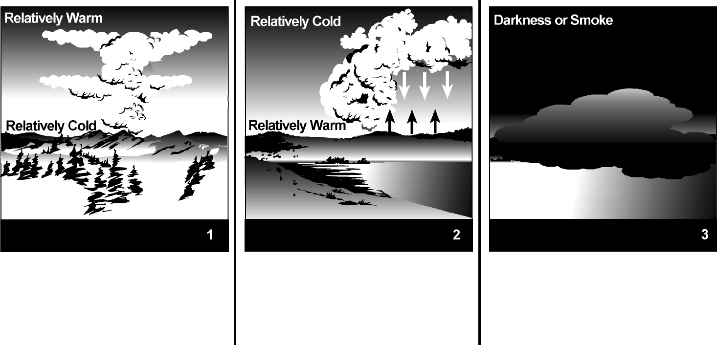
• Clouds in layers, no vertical motion • Clouds grow vertically and smoke rises to • Smoke column is not observable because

• Stratus type clouds great heights of nighttime conditions or observer’s loca-

• Smoke column drifts apart after limited rise • Cumulus type clouds tion is in smoke

• Poor visibility in lower levels due to • Upward and downward currents of gusty

accumulation of haze and smoke winds

• Fog layers • Good visibility

• Steady winds • Dust whirls

Park/Unit 4-Character Alpha Code:

FMH-4 MONITORING TYPE DESCRIPTION SHEET

Monitoring Type Code: ________________________ Date Described: / /

Monitoring Type Name:

FGDC Association(s):

Preparer(s) (FEMO/RMS/FMO):

Burn Prescription (including other treatments:

Management Objective(s):

Monitoring Objective(s):

Objective Variable(s):

Physical Description:

Biological Description:

Rejection Criteria:

Notes:

Date Entered: / /

FMH-4

FMH-4 PLOT PROTOCOLS

GENERAL PROTOCOLS (Circle One) (Circle One)

Control Treatment Plots (Opt) Y N Herb Height (Opt) Y N

Herbaceous Density (Opt) Y N Abbreviated Tags (Opt) Y N

OP/Origin Buried (Opt) Y N Herb. Fuel Load (Opt) Y N

Preburn

Voucher Specimens (Opt) Y N Brush Fuel Load (Opt)

Count Dead Branches of Living Plants as Dead (Opt)

Y

N

Width Sample Area Species Not Intercepted But Seen in Vicinity of Herbaceous

Transect(s):

Length/Width Sample Area for

Stakes Installed:

Shrubs:

Herbaceous Frame Dimensions:

Herbaceous Density Data Collected At:

Burn Duff Moisture (Opt) Y N Flame Depth (Opt) Y N

Postburn

100 Pt. Burn Severity (Opt) Y N Herb. Fuel Load (Opt) Y N

Herbaceous/Shrub Data (Opt): FMH- 15/16/17/18

FOREST PLOT PROTOCOLS (Circle One) (Circle One)

Live Tree Damage (Opt) Y N Live Crown Position (Opt) Y N

Dead Tree Damage (Opt) Y N Dead Crown Position (Opt) Y N

Overstory

(>15 cm)

Record DBH Year-1 (Opt) Y N

Length/Width of Sample Area: Quarters Sampled: Subset

w Q1 w Q2 w Q3 w Q4

Height (Opt) Y N Poles Tagged (Opt) Y N

Pole-size

Record DBH Year-1 (Opt) Y N Dead Pole Height (Opt) Y N

(>2.5<15)

Length/Width of Sample Area: Quarters Sampled: Subset

w Q1 w Q2 w Q3 w Q4

Height (Opt) Y N Seedlings Mapped (Opt) Y N

Seedling

Dead Seedlings (Opt) Y N Dead Seedling Height (Opt) Y N

(<2.5 cm)

Length/Width of Sample Area: Quarters Sampled: Subset

w Q1 w Q2 w Q3 w Q4

Fuel Load Sampling Plane Lengths:___ 1 hr

w ___ 10 hr w ___ 100 hr w ___ 1,000 hr-s w ___ 1,000 hr-r

Herbaceous Cover Data Collected at: Q4–Q1

w Q3–Q2 w 0P–50P w Q4–30 m

Postburn Char Height (Opt) Y N Poles in Assessment (Opt) Y N

Collect Severity Along: Fuel Transects

w Herbaceous Transects

(Opt) = Optional

FMH-4

Park/Unit 4-Character Alpha Code:

FMH-5 PLOT LOCATION DATA SHEET

Plot ID: B / C (Circle One) Date: / /

Burn Unit: Recorder(s):

Topo Quad: Transect Azimuth: Declination:

UTM ZONE:

Lat: Section: Slope (%) along Transect Azimuth:

UTMN: Long: Township: Slope (%) of Hillside:

UTME: Range: Aspect: Elevation:

Location Information Determined by (Circle One): Map & Compass / GPS

If determined by GPS: Datum used: (Circle One) PDOP/EHE:

Fire History of the Plot (including the date of the last known fire):

1. Road and trail used to travel to the plot:

2. True compass bearing at point where road/trail is left to hike to plot: _____°

3. Describe the route to the plot; include or attach a hand-drawn map illustrating these directions,

including the plot layout, plot reference stake and other significant features. In addition, attach a

topo, orthophoto, and/or trail map.

4. Describe reference feature: _________________________________________________________

5. True compass bearing from plot reference feature to plot reference stake: _________°

6. Distance from reference feature to reference stake: __________m

7. Problems, comments, notes:

Date Entered: / /

FMH-5

FMH-5A HISTORY OF SITE VISITS

Plot ID: B / C (Circle One) Burn Unit:

Date

Burn

Status

Purpose Comments

FMH-5A

Date Entered:

/ /

Park/Unit 4-Character Alpha Code:

FMH-6 SPECIES CODE LIST

Page of

Use this form to record unknowns and official species codes. Tip: Place an asterisk next to each species

you voucher.

Species

Code

Life

Form

Genus/Species (spell out full name)

Native

(Circle

One)

Annual/

Biennial/

Perennial

Y N

Life Forms Codes:

A Fern or Fern Ally G Grass R Grass-like T Tree * Substrate

F Forb N Non-vascular S Shrub U Subshrub V Vine

Date Entered: / /

FMH-6

VOUCHER SPECIMEN DATA COLLECTION FORMS

Date: Plot ID: Collected by: Coll. #

Latin Name: Family:

Common Name:

Description: ann/bien/per

flr. color:

fruit type:

Life form:

other:

ht.: Habitat:

Topo Quad: Assoc. spp.:

Location (

UTM, lat/long): Elev.: Slope: Aspect:

Comments:

Date: Plot ID: Collected by: Coll. #

Latin Name: Family:

Common Name:

Description: ann/bien/per

flr. color:

fruit type:

Life form:

other:

ht.: Habitat:

Topo Quad: Assoc. spp.:

Location (

UTM, lat/long): Elev.: Slope: Aspect:

Comments:

Date: Plot ID: Collected by: Coll. #

Latin Name: Family:

Common Name:

Description: ann/bien/per

flr. color:

fruit type:

Life form:

other:

ht.: Habitat:

Topo Quad: Assoc. spp.:

Location (

UTM, lat/long): Elev.: Slope: Aspect:

Comments:

Date: Plot ID: Collected by: Coll. #

Latin Name: Family:

Common Name:

Description: ann/bien/per

flr. color:

fruit type:

Life form:

other:

ht.: Habitat:

Topo Quad: Assoc. spp.:

Location (

UTM, lat/long): Elev.: Slope: Aspect:

Comments:

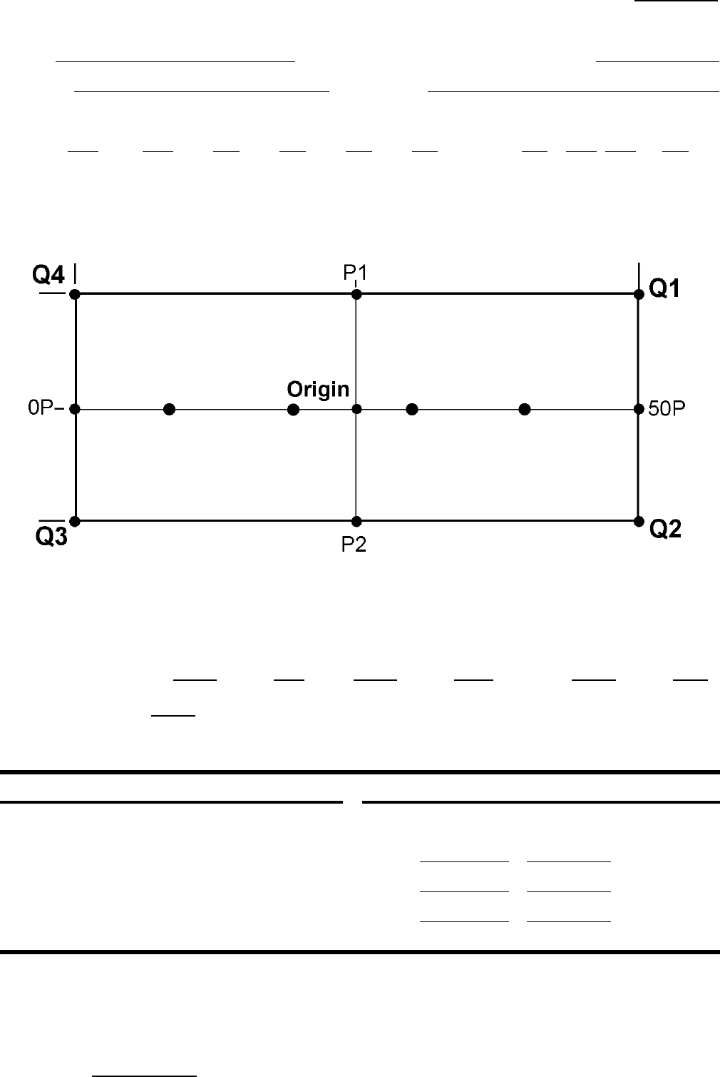
Park/Unit 4-Character Alpha Code:

FMH-7 FOREST PLOT DATA SHEET

Plot ID:

Burn Unit:

B / C (Circle One)

Recorders:

Date: / /

Burn Status:Circle one and indicate number of times treated, e.g., 01-yr01, 02-yr01

00-PRE Post -yr01 -yr02 -yr05 -yr10 -yr20Other: -yr ; -mo

Overstory: m

2

in Q Pole: m

2

in Q Seedling: m

2

in Q

Sampling

Shrub: m

2

along Q4–Q1 w Q3–Q2 w 0P–50P w Q4–30 m

Areas:

Shade in the sampling areas for each tree class and for the shrub sampling area(s) on the

plot layout above.

Photo Subject Order Fuel Load Transects

1. 0P

Ł Origin 6. Q2 Ł Q3 Azimuth Slope

2. Q4

Ł Q1 7. P2 Ł Origin 1

3. P1

Ł Origin 8. Q3 Ł Q2 2

4. Q1

Ł Q4 9. Origin Ł REF 3

5. 50P

Ł Origin 10. REF Ł Origin 4

Record photo documentation data for each visit Draw in fuel load transect lines on the plot layout

on FMH-23, Photographic record sheet above.

Date Entered: / /

FMH-7

Park/Unit 4-Character Alpha Code:

FMH-8 OVERSTORY TAGGED TREE DATA SHEET

Page of

Plot ID: B / C (Circle One) Date: / /

Burn Unit: Recorders:

Burn Status:Circle one and indicate number of times treated, e.g., 01-yr01, 02-yr01

00-PRE Post -yr01 -yr02 -yr05 -yr10 -yr20Other: -yr ; -mo

Record: quarter (Qtr), tag #, species by code (Spp), DBH in centimeters, live/dead, crown position code

(CPC, Optional), damage code (Damage, Optional), and provide any helpful comments for data analysts

or future monitors (Comments).

Qtr Tag Spp

DBH

(cm)

Live CPC Damage (codes below) Comments

Y N

Crown Position Codes (CPC) Note: Codes 10–12 are only used postburn, e.g., 01-yr01, 01-yr02, etc., and only used once:

1 Dominant 2 Co-dominant 3 Intermediate 4 Subcanopy

5 Open Growth / Isolated 6 Recent Snag 7 Loose Bark Snag 8 Clean Snag

9 Broken above BH 10 Broken below BH 11 Dead and down 12 Cut Stump

Damage Codes:

ABGR—Abnormal CONK—Large Shelf FIRE—Fire Scar / INSE—Insects / MISL—Mistletoe SPAR—Unusually Sparse

Growth Fungus Cambial Damage Their Sign Foliage

BIRD—e.g., Sapsucker CROK—Crooked Bole FORK—Forked Top LEAN—Leaning Tree MOSS—Moss SPRT—Sprouts at Base

BLIG—Blight DTOP—Dead Top FRST—Frost Crack LICH—Lichen OZON—Ozone TWIN—Twin–below DBH

BROK—Broken Top EPIC—Sprouts from GALL—Galls LIGT—Lightning ROOT—Large UMAN—Human-caused

Bole / Limbs Scar Exposed Roots Damage

BROM—Witches’ EPIP—Epiphytes HOLW—Hollowed-out MAMM—Mammal ROTT—Rot / Fungus WOND—Wound–cracks

Broom Damage Other than Conk

BURL—Burl

Date Entered: / /

FMH-8

Qtr Tag Spp

DBH

(cm)

Live CPC Damage Comments

Y N

FMH-8

Park/Unit 4-Character Alpha Code:

FMH-9 POLE-SIZE TREE DATA SHEET

Page of

Plot ID: B / C (Circle One) Date: / /

Burn Unit: Recorders:

Burn Status:Circle one and indicate number of times treated, e.g., 01-yr01, 02-yr01

00-PRE Post -yr01 -yr02 -yr05 -yr10 -yr20Other: -yr ; -mo

Record: quarter (if other than Q1), tag # (Optional), species by code (Spp), DBH in centimeters, live/

dead, and height by code (Hgt, Optional).

Qtr

Tag or

Map#

Spp

DBH

(cm)

Live

Hgt

Code

Qtr

Tag or

Map#

Spp

Y N

DBH

(cm)

Live

Hgt

Code

Y N

Height Class Codes (height in centimeters):

1 0–15 5 100.1–200 9 500.1–600

2

3

15.1–30

30.1–60

6

7

200.1–300

300.1–400

10

11

600.1–700

700.1–800

13 900.1+

4 60.1–100 8 400.1–500 12 800.1–900

Note: Measure height from ground level to the highest point of growth on the tree. The highest point on

a bent tree would be down the trunk of the tree instead of at the growing apex. Only use height codes 1-

4 for leaning trees.

Date Entered: / /

FMH-9

Qtr

Tag or

Map#

Spp

DBH

(cm)

Live

Hgt

Code

Qtr

Tag or

Map#

Spp

DBH

(cm)

Live

Hgt

Code

Y N Y N

FMH-9

Park/Unit 4-Character Alpha Code:

FMH-10 SEEDLING TREE DATA SHEET

Page of

Plot ID: B / C (Circle One) Date: / /

Burn Unit: Recorders:

Burn Status:Circle one and indicate number of times treated, e.g., 01-yr01, 02-yr01

00-PRE Post -yr01 -yr02 -yr05 -yr10 -yr20Other: -yr ; -mo

Record: map number (Map#, Optional), species code (Spp), live/dead, height by class (Hgt Code,

Optional), resprout (Rsprt), and # by species and height class (Num/Tally).

Area Sampled: in Quarter(s):

Map# Spp Live

Hgt

Code

Rsprt Num/Tally Map# Spp Live

Hgt

Code

Rsprt Num/Tally

Y N Y N Y N Y N

Height Class Codes (height in centimeters)

1 0–15 5 100.1–200 9 500.1–600

2

3

15.1–30

30.1–60

6

7

200.1–300

300.1–400

10

11

600.1–700

700.1–800

13 900.1+

4 60.1–100 8 400.1–500 12 800.1–900

Note: Measure height from ground level to the highest point of growth on the tree. The highest point on

a bent tree would be down the trunk of the tree instead of at the growing apex.

Date Entered: / /

FMH-10

Park/Unit 4-Character Alpha Code:

FMH-10A ALTERNATE SEEDLING TREE DATA SHEET

Page of

Plot ID: B / C (Circle One) Date: / /

Burn Unit: Recorders:

Burn Status:Circle one and indicate number of times treated, e.g., 01-yr01, 02-yr01

00-PRE Post -yr01 -yr02 -yr05 -yr10 -yr20Other: -yr ; -mo

Record: map number (Map#, Optional), species code (Spp), live/dead, height by class (Hgt, Optional),

resprout (Rsprt), and # by species and height class (Num/Tally).

Area Sampled: in Quarter(s):

Map# Spp Live

Hgt

Code

Rsprt Num Tally

Y N Y N

Height Class Codes (height in centimeters)

1 0–15 5 100.1–200 9 500.1–600

2

3

15.1–30

30.1–60

6

7

200.1–300

300.1–400

10

11

600.1–700

700.1–800

13 900.1+

4 60.1–100 8 400.1–500 12 800.1–900

Note: Measure height from ground level to the highest point of growth on the tree. The highest point on

a bent tree would be down the trunk of the tree instead of at the growing apex.

FMH-10A

Date Entered:

/ /

Park/Unit 4-Character Alpha Code:

y

FMH-11 FULL PLOT TREE MAP

Plot ID: B/C (Circle One) Date: / /

Burn Unit: Recorders:

Burn Status:Circle one and indicate number of times treated, e.g., 01-yr01, 02-yr01

00-PRE Post -yr01 -yr02 -yr05 -yr10 -yr20 Other: -yr ; -mo

5 m 10 m 15 m 20 m

Tree Class

50 m

0 m

(Circle One)

45 m

Overstory

Pole

40 m

Seedling

35 m

30 m

25m

(P1)

20 m

15 m

10 m

5 m

0 m

4A

Q 1 Q 2

3A

P2

2A

Q 4 Q 3

1A

FMH-11

Park/Unit 4-Character Alpha Code:

FMH-12 QUARTER PLOT TREE MAP

Plot ID: B/C (Circle One) Date: / /

Burn Unit: Recorders:

Burn Status:Circle one and indicate number of times treated, e.g., 01-yr01, 02-yr01

00-PRE Post -yr01 -yr02 -yr05 -yr10 -yr20 Other: -yr ; -mo

Tree Class

(Circle One)

Overstory

Pole

Seedling

m

0 m

5 m 10 m

m

25m 25m

m

FMH-12

Park/Unit 4-Character Alpha Code:

FMH-13 ALTERNATE TREE MAP

Plot ID: B/C (Circle One) Date:

Burn Unit: Recorders:

Burn Status:Circle one and indicate number of times treated, e.g., 01-yr01, 02-yr01

00-PRE Post -yr01 -yr02 -yr05 -yr10 -yr20 Other: -yr

Tree Class m

m m

;

/ /

-mo

m

(Circle One)

Overstory

Pole

m

Seedling

m

FMH-13

Park/Unit 4-Character Alpha Code:

FMH-14

50 m

2

TREE MAP

Plot ID: B/C (Circle One) Date: / /

Burn Unit: Recorders:

Burn Status:Circle one and indicate number of times treated, e.g., 01-yr01, 02-yr01

00-PRE Post -yr01 -yr02 -yr05 -yr10 -yr20 Other: -yr ; -mo

(P1)

25 m 27.5 m 30 m

Tree Class

0 m

(Circle One)

2.5 m

Overstory

Pole

5 m

Seedling

7.5 m

10 m

(Origin) 30 m (3A)

FMH-14

Park/Unit 4-Character Alpha Code:

FMH-15 50 m TRANSECT DATA SHEET

Plot ID: B/C (Circle One) Date: / /

Burn Unit: Recorders:

Burn Status:Circle one and indicate number of times treated, e.g., 01-yr01, 02-yr01

00-PRE Post -yr01 -yr02 -yr05 -yr10 -yr20Other: -yr ; -mo

Phenological Stage: (Circle One) Q4–Q1

w Q3–Q2 w 0P–50P

Pnt Tape Hgt (m) Spp; Species or Substrate Codes (tallest to lowest)

1 0.3

2 0.6

3 0.9

4 1.2

5 1.5

6 1.8

7 2.1

8 2.4

9 2.7

10 3.0

11 3.3

12 3.6

13 3.9

14 4.2

15 4.5

16 4.8

17 5.1

18 5.4

19 5.7

20 6.0

21 6.3

22 6.6

23 6.9

24 7.2

25 7.5

26 7.8

27 8.1

28 8.4

29 8.7

30 9.0

31 9.3

32 9.6

33 9.9

34 10.2

35 10.5

36 10.8

37 11.1

Date Entered: / / FMH-15

Plot ID: Date: / / (Circle One) Q4–Q1 • Q3–Q2 • 0P–50P

Pnt Tape Hgt (m) Spp; Species or Substrate Codes (tallest to lowest)

38 11.4

39 11.7

40 12.0

41 12.3

42 12.6

43 12.9

44 13.2

45 13.5

46 13.8

47 14.1

48 14.4

49 14.7

50 15.0

51 15.3

52 15.6

53 15.9

54 16.2

55 16.5

56 16.8

57 17.1

58 17.4

59 17.7

60 18.0

61 18.3

62 18.6

63 18.9

64 19.2

65 19.5

66 19.8

67 20.1

68 20.4

69 20.7

70 21.0

71 21.3

72 21.6

73 21.9

74 22.2

75 22.5

76 22.8

77 23.1

78 23.4

79 23.7

80 24.0

81 24.3

FMH-15

Plot ID: Date: / / (Circle One) Q4–Q1 • Q3–Q2 • 0P–50P

Pnt Tape Hgt (m) Spp; Species or Substrate Codes (tallest to lowest)

82 24.6

83 24.9

84 25.2

85 25.5

86 25.8

87 26.1

88 26.4

89 26.7

90 27.0

91 27.3

92 27.6

93 27.9

94 28.2

95 28.5

96 28.8

97 29.1

98 29.4

99 29.7

100 30.0

101 30.3

102 30.6

103 30.9

104 31.2

105 31.5

106 31.8

107 32.1

108 32.4

109 32.7

110 33.0

111 33.3

112 33.6

113 33.9

114 34.2

115 34.5

116 34.8

117 35.1

118 35.4

119 35.7

120 36.0

121 36.3

122 36.6

123 36.9

124 37.2

125 37.5

FMH-15

Pnt Tape Hgt (m) Spp; Species or Substrate Codes (tallest to lowest)

126 37.8

127 38.1

128 38.4

129 38.7

130 39.0

131 39.3

132 39.6

133 39.9

134 40.2

135 40.5

136 40.8

137 41.1

138 41.4

139 41.7

140 42.0

141 42.3

142 42.6

143 42.9

144 43.2

145 43.5

146 43.8

147 44.1

148 44.4

149 44.7

150 45.0

151 45.3

152 45.6

153 45.9

154 46.2

155 46.5

156 46.8

157 47.1

158 47.4

159 47.7

160 48.0

161 48.3

162 48.6

163 48.9

164 49.2

165 49.5

166 49.8

Species observed within ___ m of either side of the transect but not intercepted:

FMH-15

Park/Unit 4-Character Alpha Code:

FMH-16 30 m TRANSECT DATA SHEET

Plot ID: B/C (Circle One) Date: / /

Burn Unit: Recorders:

Burn Status:Circle one and indicate number of times treated, e.g., 01-yr01, 02-yr01

00-PRE Post -yr01 -yr02 -yr05 -yr10 -yr20Other: -yr ; -mo

Phenological Stage: (Circle One) Q4–30 m

w 0P–30P

Pnt Tape Hgt (m) Spp; Species or Substrate Codes (tallest to lowest)

1 0.3

2 0.6

3 0.9

4 1.2

5 1.5

6 1.8

7 2.1

8 2.4

9 2.7

10 3.0

11 3.3

12 3.6

13 3.9

14 4.2

15 4.5

16 4.8

17 5.1

18 5.4

19 5.7

20 6.0

21 6.3

22 6.6

23 6.9

24 7.2

25 7.5

26 7.8

27 8.1

28 8.4

29 8.7

30 9.0

31 9.3

32 9.6

33 9.9

34 10.2

35 10.5

36 10.8

37 11.1

38 11.4

39 11.7

40 12.0

41 12.3

42 12.6

43 12.9

44 13.2

45 13.5

46 13.8

47 14.1

Date Entered: / / FMH-16

Pnt Tape Hgt (m) Spp; Species or Substrate Codes (tallest to lowest)

48 14.4

49 14.7

50 15.0

51 15.3

52 15.6

53 15.9

54 16.2

55 16.5

56 16.8

57 17.1

58 17.4

59 17.7

60 18.0

61 18.3

62 18.6

63 18.9

64 19.2

65 19.5

66 19.8

67 20.1

68 20.4

69 20.7

70 21.0

71 21.3

72 21.6

73 21.9

74 22.2

75 22.5

76 22.8

77 23.1

78 23.4

79 23.7

80 24.0

81 24.3

82 24.6

83 24.9

84 25.2

85 25.5

86 25.8

87 26.1

88 26.4

89 26.7

90 27.0

91 27.3

92 27.6

93 27.9

94 28.2

95 28.5

96 28.8

97 29.1

98 29.4

99 29.7

100 30.0

Species observed within ___ m of either side of the transect but not intercepted:

FMH-16

Park/Unit 4-Character Alpha Code:

FMH-17 SHRUB DENSITY DATA SHEET

Page of

Plot ID: B / C (Circle One) Date: / /

Burn Unit: Recorders:

Burn Status:Circle one and indicate number of times treated, e.g., 01-yr01, 02-yr01

00-PRE Post -yr01 -yr02 -yr05 -yr10 -yr20Other: -yr ; -mo

Transect: Q4–Q1

w Q3–Q2 w 0P–50P w Q4–30 m w 0P–30P (Circle One)

For living and dead plants within the transect, count each individual having >50% of its rooted base in

the belt. The optional interval field (Int) can be used to divide the belt into subunits to facilitate species

counts. Record Age Class (Age) code (see below).

Belt Width: m Length: m Side of transect monitored facing 30P (Brush Plots Only):

Int Spp Age Live Num / Tally Int Spp Age Live Num / Tally

Y N Y N

A g e C l a s s C o d e s :

I

Immature–Seedling

R

Resprout

M

Mature–Adult

Date Entered: / / FMH-17

Park/Unit 4-Character Alpha Code:

FMH-17A

Plot ID:

Burn Unit:

ALTERNATE SHRUB DENSITY DATA SHEET

B / C (Circle One)

Recorders:

Date:

Page

/

of

/

Burn Status:Circle one and indicate number of times treated, e.g., 01-yr01, 02-yr01

00-PRE Post -yr01 -yr02 -yr05 -yr10 -yr20Other: -yr ; -mo

Transect: Q4–Q1

w Q3–Q2 w 0P–50P w Q4–30 m w 0P–30P (Circle One)

For living and dead plants within the transect, count each individual having >50% of its rooted base in

the belt. The optional interval field (Int) can be used to divide the belt into subunits to facilitate species

counts. Record Age Class (Age) code (see below).

Belt Width: m Length: m Side of transect monitored facing 30P (Brush Plots Only):

Int Spp Age Live Num Tally

Y N

Age Class Codes:

I

Immature–Seedling

R

Resprout

M

Mature–Adult

FMH-17A

Date Entered:

/ /

Park/Unit 4-Character Alpha Code:

FMH-18 HERBACEOUS DENSITY DATA SHEET

Plot ID: B / C (Circle One)

Burn Unit: Recorders:

Burn Status:Circle one and indicate number of times treated, e.g., 01-yr01, 02-yr01

00-PRE Post -yr01 -yr02 -yr05 -yr10 -yr20Other:

Date:

-yr ;

Page

/

-mo

of

/

Transect: Q4–Q1

w Q3–Q2 w 0P–50P w Q4–30 m w 0P–30P (Circle One)

For living and dead plants within the transect, count each individual having >50% of its rooted base in

the sampling area.

Frame Size: m

2

Side of transect m onitored facing 30P (Brush Plots Only ):

Frame # Spp Live Num Frame # Spp Live Num

Y N Y N

Date Entered: / / FMH-18

Frame # Spp Live Num Frame # Spp Live Num

Y N

FMH-18

Y N

Park/Unit 4-Character Alpha Code:

FMH-19 FOREST PLOT FUELS INVENTORY DATA SHEET

Page of

Plot ID: B / C (Circle One) Date: / /

Burn Unit: Recorders:

Burn Status:Circle one and indicate number of times treated, e.g., 01-yr01, 02-yr01

00-PRE Post -yr01 -yr02 -yr05 -yr10 -yr20Other: -yr ; -mo

Transect lengths, in feet: 0-0.25: 0.25-1: 1-3: 3+s: 3+r:

0–.25” .25–1” 1–3” 3+s 3+r

Transect 1

Compass

Dir._____°

Slope___%

Tag 1A

& 1B

Transect 2

Compass

Dir._____°

Slope___%

Tag 2A

& 2B

Transect 3

Compass

Dir._____°

Slope___%

Tag 3A

& 3B

Transect 4

Compass

Dir._____°

Slope___%

Tag 4A

& 4B

(1-hr)

(10-hr) (100-hr) (1,000-hr)

1 25

5 30

10 35

15 40

20 45

1 25

5 30

10 35

15 40

20 45

1 25

5 30

10 35

15 40

20 45

1 25

5 30

10 35

15 40

20 45

# of intercepts Diameter (in) Litter and Duff Depths (in)

L D L D

Note: See reverse for definitions and tally rules

Date Entered: / / FMH-19

FMH-19

Definitions

Litter—Includes freshly fallen leaves, needles, bark, flakes, fruits (e.g., acorns, cones), cone scales,

dead matted grass, and a variety of miscellaneous vegetative parts. Does not include twigs and larger

stems.

Duff—The fermentation and humus layers; does not include the freshly cast material in the litter layer,

nor in the postburn environment, ash. The top of the duff is where needles, leaves, fruits and other cast-

off vegetative material have noticeably begun to decompose. Individual particles usually are bound by

fungal mycelia. The bottom of the duff is mineral soil.

Downed Woody Material—Dead twigs, branches, stems and boles of trees and shrubs that have fallen

and lie on or above the ground.

Obstructions Encountered Along Fuel Transects—If the fuel transect azimuth goes directly through a

rock or stump, in most cases you can run the tape up and over it. If the obstruction is a tree, go around it

and pick up the correct azimuth on the other side. Be sure to note on the FMH-19 on which side of the

bole the tape deviated so that it will be strung the same way in the future.

Litter and Duff Measurement Rules

• If the transect is longer than 50 ft, do not take additional litter and duff measurements.

• Do not take measurements at the stake (0 point); it is an unnatural structure that traps materials.

• At each sampling point, gently insert a trowel or knife into the ground, until you hit mineral soil, then

carefully pull it away exposing the litter/duff profile. Locate the boundary between the litter and duff

layers. Vertically measure the litter and duff to the nearest tenth of an inch.

• Refill holes created by this monitoring technique.

• Do not include twigs and larger stems in litter depth measurements.

• Occasionally moss, a tree trunk, stump, log, or large rock will occur at a litter or duff depth data col-

lection point. If moss is present, measure the duff from the base of the green portion of the moss. If a

tree, stump or large rock is on the point, record the litter or duff depth as zero, even if there is litter or

duff on top of the stump or rock.

• If a log is in the middle of the litter or duff measuring point, move the data collection point one foot

over to the right, perpendicular to the sampling plane.

Tally Rules for Downed Woody Material

• Measure woody material first to avoid disturbing it and biasing your estimates.

• Do not count dead woody stems and branches still attached to standing shrubs and trees.

• Do not count twigs and branches when the intersection between the central axis of the particle and

the sampling plane lies in the duff.

• If the sampling plane intersects the end of a piece, tally only if the central axis is crossed.

• Do not tally any particle having a central axis that coincides perfectly with the sampling plane.

• If the sampling plane intersects a curved piece more than once, tally each intersection.

• Tally uprooted stumps and roots not encased in dirt. Do not tally undisturbed stumps.

• For rotten logs that have fallen apart, visually construct a cylinder containing the rotten material and

estimate its diameter.

• When stumps, logs, and trees occur at the point of measurement, offset 1 ft (0.3 m) perpendicular to

the right side of the sampling plane.

• Measure through rotten logs whose central axis is in the duff layer.

Park/Unit 4-Character Alpha Code:

FMH-20 TREE POSTBURN ASSESSMENT DATA SHEET Page of

Plot ID: B / C (Circle One) Date: / /

Burn Unit: Recorders:

Burn Status:Circle one and indicate number of times treated, e.g., 01-Post, 02-Post) Post

For each tagged tree record: Tag #, tree status (Live Code) (see below), maximum scorch height

(ScHgt), percent crown scorched (ScPer), and char height (Char) (Optional).

Overstory

w

ww

w Pole (Circle One)

Tag

Live

Code

ScHgt

(m)

ScPer

Char

(m)

Tag

Live

Code

ScHgt

(m)

ScPer

Char

(m)

Live Codes:

LLive DDead R Resprouting C Consumed/Down B Broken below DBH SCut Stump

Notes: :

Date Entered: / / FMH-20

Overstory w

ww

w Pole (Circle One)

Tag

Live

Code

ScHgt

(m)

ScPer

Char

(m)

Tag

Live

Code

ScHgt

(m)

ScPer

Char

(m)

FMFMH-2H-200

Park/Unit 4-Character Alpha Code:

FMH-21 FOREST PLOT BURN SEVERITY DATA SHEET Page of

Plot ID: B / C (Circle One) Date: / /

Burn Unit: Recorders:

Burn Status:Circle one and indicate number of times treated, e.g., 01-Post, 02-Post) Post

When collecting burn severity on fuel transects, rate each fuel load transect at the duff measurement

points using the Coding Matrix below. When collecting burn severity on herbaceous transects, rate each

herbaceous transect (Q4–Q1—transect 1, Q3–Q2—transect 2, 0P–50P—transect 3) at the meter mea-

surement points on the tape listed in the tables below (1, 5, 10, etc.) using the same matrix. Collect data

only along the transects where you collected preburn data. Note: If you read only herbaceous transect

Q4–30 m, use FMH-22.

Each observation is from a 4 dm

2

area.

Transect 1 1 5 10 15 20 25 30 35 40 45

Vegetation

Substrate

Transect 2 1 5 10 15 20 25 30 35 40 45

Vegetation

Substrate

Transect 3 1 5 10 15 20 25 30 35 40 45

Vegetation

Substrate

Transect 4 1 5 10 15 20 25 30 35 40 45

Vegetation

Substrate

Coding Matrix:

5 Unburned 4 Scorched 3 Lightly Burned 2 Moderately Burned 1 Heavily Burned 0 Not Applicable

Note: See reverse for detailed definitions.

Date Entered: / / FMH-21

FMH-21

Unburned

(5)

Scorched

(4)

Lightly Burned

(3)

Moderately Burned

(2)

Heavily Burned

(1)

Not

Applicable

(0)

Substrate

(S)

not burned litter partially blackened;

duff nearly unchanged;

wood/leaf structures

unchanged

litter charred to partially

consumed; upper duff layer

may be charred but the duff

layer is not altered over the

entire depth; surface

appears black; woody

debris is partially burned;

logs are scorched or

blackened but not charred;

rotten wood is scorched to

partially burned

litter mostly to entirely

consumed, leaving coarse,

light colored ash; duff

deeply charred, but

underlying mineral soil is

not visibly altered; woody

debris is mostly consumed;

logs are deeply charred,

burned-out stump holes are

common

litter and duff completely

consumed, leaving fine

white ash; mineral soil

visibly altered, often

reddish; sound logs are

deeply charred, and rotten

logs are completely

consumed. This code

generally applies to less

than 10% of natural or slash

burned areas

inorganic

preburn

Vegetation

(V)

not burned foliage scorched and

attached to supporting

twigs

foliage and smaller twigs

partially to completely

consumed; branches

mostly intact

foliage, twigs, and small

stems consumed; some

branches still present

all plant parts consumed,

leaving some or no major

stems/trunks; any left are

deeply charred

none present

preburn

Park/Unit 4-Character Alpha Code:

FMH-22 BRUSH AND GRASSLAND PLOT BURN SEVERITY DATA SHEET Page of

Plot ID: B / C (Circle One) Date: / /

Burn Unit: Recorders:

Burn Status:Circle one and indicate number of times treated, e.g., 01-Post, 02-Post) Post

Burn severity ratings are made every 5 m using the Coding Matrix below. Each observation is from a 4

dm

2

area (top form). Optionally, you can use the lower form, which will allow you to rate severity at all

100 points. Note: If your herbaceous transect(s) are longer than 30 m, use FMH-21.

(Circle One) Q4–30 m

w 0P–30P

1 m 5 m 10 m 15 m 20 m 25 m 30 m

Vegetation

Substrate

––––––––––––––––––––––––––––––––––––––– OR –––––––––––––––––––––––––––––––––––––

Substrate and Vegetation Burn Severity at Every Point (Optional)

0.3 S V 6.3 S V 12.3 S V 18.3 S V 24.3 S V

0.6 S V 6.6 S V 12.6 S V 18.6 S V 24.6 S V

0.9 S V 6.9 S V 12.9 S V 18.9 S V 24.9 S V

1.2 S V 7.2 S V 13.2 S V 19.2 S V 25.2 S V

1.5 S V 7.5 S V 13.5 S V 19.5 S V 25.5 S V

1.8 S V 7.8 S V 13.8 S V 19.8 S V 25.8 S V

2.1 S V 8.1 S V 14.1 S V 20.1 S V 26.1 S V

2.4 S V 8.4 S V 14.4 S V 20.4 S V 26.4 S V

2.7 S V 8.7 S V 14.7 S V 20.7 S V 26.7 S V

3.0 S V 9.0 S V 15.0 S V 21.0 S V 27.0 S V

3.3 S V 9.3 S V 15.3 S V 21.3 S V 27.3 S V

3.6 S V 9.6 S V 15.6 S V

21.6 S V 27.6 S V

3.9 S V 9.9 S V 15.9 S V 21.9 S V 28.9 S V

4.2 S V 10.2 S V 16.2 S V 22.2 S V 28.2 S V

4.5 S V 10.5 S V 16.5 S V 22.5 S V 28.5 S V

4.8 S V 10.8 S V 16.8 S V 22.8 S V 29.8 S V

5.1 S V 11.1 S V 17.1 S V 23.1 S V 29.1 S V

5.4 S V 11.4 S V 17.4 S V 23.4 S V 29.4 S V

5.7 S V 11.7 S V 17.7 S V 23.7 S V 29.7 S V

6.0 S V 12.0 S V 18.0 S V 24.0 S V 30.0 S V

Coding Matrix:

5 Unburned 4 Scorched 3 Lightly Burned 2 Moderately Burned 1 Heavily Burned 0 Not Applicable

Note: See reverse for detailed definitions.

Date Entered: / / FMH-22

Shrublands Grasslands

Substrate

(S)

Vegetation

(V)

Substrate

(S)

Vegetation

(V)

Unburned

(5)

not burned not burned

litter partially foliage scorched and

not burned not burned

litter partially foliage scorched Scorched

(4) blackened; duff nearly

unchanged; wood/leaf

structures unchanged

attached to

supporting twigs

litter charred to

foliage and smaller

blackened; duff nearly

unchanged; leaf

structures unchanged

litter charred to

grasses with

Lightly

Burned partially consumed,

twigs partially to

partially consumed,

approximately two

(3) some leaf structure

undamaged; surface

is predominately

black; some gray ash

may be present

immediately

postburn; charring

may extend slightly

into soil surface

where litter is sparse,

otherwise soil is not

altered

completely

consumed; branches

mostly intact; less

than 60% of the shrub

canopy is commonly

consumed

leaf litter consumed,

leaving coarse, light

colored ash; duff

deeply charred, but

underlying mineral

soil is not visibly

altered; woody debris

is mostly consumed;

logs are deeply

charred, burned-out

stump holes are

common

foliage, twigs, and

small stems

consumed; some

branches (>.6–1 cm in

diameter) (0.25–0.50

in) still present; 40–

80% of the shrub

canopy is commonly

consumed

leaf litter completely

all plant parts

but some plant parts

are still discernible;

charring may extend

slightly into soil

surface, but soil is not

visibly altered;

surface appears black

(this soon becomes

inconspicuous);

burns may be spotty

to uniform depending

on the grass

continuity

inches of stubble;

foliage and smaller

twigs of associated

species partially to

completely

consumed; some

plant parts may still be

standing; bases of

plants are not deeply

burned and are still

recognizable

leaf litter consumed,

leaving coarse, light

gray or white colored

ash immediately after

the burn; ash soon

disappears leaving

bare mineral soil;

charring may extend

slightly into soil

surface

unburned grass

stubble usually less

than 2 in tall, and

mostly confined to an

outer ring; for other

species, foliage

completely

consumed, plant

bases are burned to

ground level and

obscured in ash

immediately after

burning; burns tend to

be uniform

leaf litter completely

no unburned grasses

Moderately

Burned

(2)

Heavily

Burned consumed, leaving a

consumed leaving consumed, leaving a

above the root crown;

(1) fluffy fine white ash;

all organic material is

consumed in mineral

soil to a depth of 1–2.5

cm (0.5–1 in), this is

underlain by a zone of

black organic

material; colloidal

structure of the

surface mineral soil

may be altered

only stubs greater

than 1 cm (0.5 in) in

diameter

inorganic preburn none present preburn

fluffy fine white ash,

this soon disappears

leaving bare mineral

soil; charring extends

to a depth of 1 cm (0.5

in) into the soil; this

severity class is

usually limited to

situations where

heavy fuel load on

mesic sites has

burned under dry

conditions and low

wind

for other species, all

plant parts consumed,

leaving some or no

major stems or

trunks, any left are

deeply charred; this

severity class is

uncommon due to the

short burnout time of

grasses

inorganic preburn none present preburn Not

Applicable

(0)

FMH-22

Park/Unit 4-Character Alpha Code:

FMH-23 PHOTOGRAPHIC RECORD SHEET

Roll ID: Brand and Type of Film:

Camera Type: Lens: m m ASA:

#

Fire Name/

Number

Plot ID

Subject

(e.g., Q3–Q2)

Azmth Date Time F-Stop S- Speed

1

2

3

4

5

6

7

8

9

10

11

12

13

14

15

16

17

18

19

20

21

22

23

24

25

26

27

28

29

30

31

32

33

34

35

36

37

38

FMH-23

Park/Unit 4-Character Alpha Code:

FMH-24 QUALITY CONTROL CHECKLIST

Plot ID:

Burn Status, e.g., 01-yr01, 02-yr01: - - - - - -

Comments:

Initials/ Initials/ Initials/ Initials/ Initials/ Initials/

Date Date Date Date Date Date

30/50 m

Transect

Data Collected

Quality Checked

Data Entered

Quality Checked

Overstory

Trees

Data Collected

Quality Checked

Data Entered

Quality Checked

Pole-size

Trees

Data Collected

Quality Checked

Data Entered

Quality Checked

Seedling

Trees

Data Collected

Quality Checked

Data Entered

Quality Checked

Fuel

Transects

Data Collected

Quality Checked

Data Entered

Quality Checked

Shrub

Density

Data Collected

Quality Checked

Data Entered

Quality Checked

Photographs Ta ken

Developed

Labeled

Data Entry Computer(s) Used

Plot Location Data Sheet

Plot Location Map

Tags

Completed?

Attached?

Quality Checked?

Offsite Data

Storage? Location:

FMH-24

Park/Unit 4-Character Alpha Code:

FMH-25 PLOT MAINTENANCE LOG

Plot ID: Date Log Initiated: ___________________

Date/

Initials

Problem Description Corrective Action

Date Completed/

Initials

Comments

FMH-25

Park/Unit 4-Character Alpha Code:

FMH-26 DATA ANALYSIS RECORD

Date: / /

Monitoring Type Information (One type per data analysis worksheet) B / C (Circle One)

Monitoring Type Code Monitoring Type Name

# Plots in this

Analysis

Resource Management Goal(s) for this Monitoring Type; e.g., restore and then maintain

naturally functioning oak savannas:

Target/Threshold Condition(s) for this Monitoring Type:

Management Objectives for this Monitoring Type; e.g., reduce total fuel load by 20-80%

immediately postburn:

Monitoring Objectives for this Monitoring Type; e.g., 80% confident of being within 25% of the

true mean fuel load:

Objective Variables Other Variables of Interest

FMH-26

—

-

—

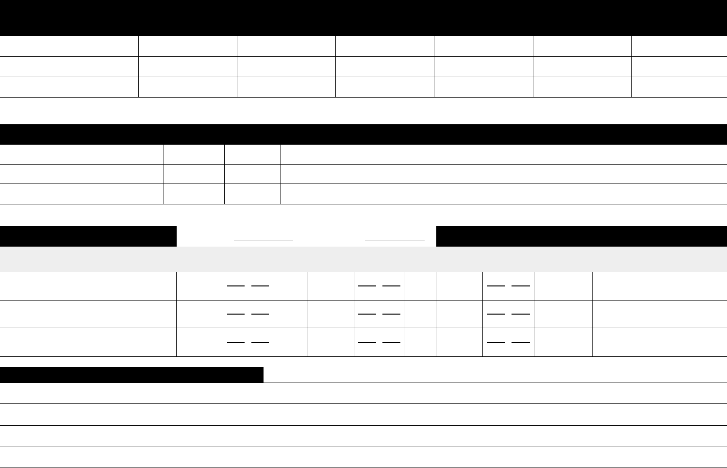
Calculated Minimum Number of Plots (Attach computer-generated printouts from which data results were obtained.)

Objective Variable

Minimum

Detectable

Change

Precision (R) or

Power (β)

Confidence

Interval (%)

Minimum

# Plots

Mean

Standard

Deviation

1.

2.

3.

Reaction/Planned Actions Based on Calculated Minimum Number of Plots

Objective Variable

Accept # plots

calculated?

Add plots &

recalculate?

Number of plots needed is prohibitive the following actions will be taken instead

1.

Yes No Ye s No

2. Yes No Yes No

3. Yes No Yes No

Change Over Any Amount of Time (Attach computer generated printouts and graphics from which results/conclusions were drawn.)

Time Period: Time Period:

SE/SD

1.

to

80/90/95

to

80/90/95

to

80/90/95

2.

to

80/90/95

to

80/90/95

to

80/90/95

3.

to

80/90/95

to

80/90/95

to

80/90/95

Objective Variable

% Change (+ or )

Objective Objective Not Met These Actions

Met? Will Be Taken

SE/SD

Actual Actual Actual

CI (%)

(circle

CI (%)

(circle

CI (%)

Value Value Value

one) one)

Discussion (add additional sheets, as necessary):

FMH-26; page 2 of 2

3

Random Nu mber Generators

B

Random Number Generators

“The generation of random numbers is too important to be left to chance.”

—Robert Coveyou

Random numbers are used to select truly random sam-

ples in monitoring plots and for other purposes. They

can be obtained from a table or by using a computer.

Note that many calculators also include random num-

ber generators.

USING A TABLE

For each use of the random number table (Table 31,

page 190) choose an arbitrary starting point within the

table, a reading direction, and a rule for continuing the

reading of numbers if the edge of the table is reached.

Number sequences may be read in any arbitrary direc-

tion (forwards horizontal, downwards vertical, diago-

nal, etc.) from the starting point, as long as this

direction is chosen without reference to placement of

numbers in the table. Various rules for continuation of

reading can be used; the easiest rules use the initial

reading direction, but give a new starting point for fur-

ther reading. The continuation rule should indicate a

new starting position relative to the table edge which

has been reached and should change that portion of

the table used for continuation reading. Suggested

continuation rules follow:

• Start at the opposite end of the table and move to

the next line (up or down)

• Start at the center of the next row above and

move in the opposite direction

Mark sequences of numbers as you read them, and

choose a unique starting point for each new use of the

table. If the chosen starting point and reading direction

have been previously used, select another point-direc-

tion combination.

To generate short sequences, such as groups of three

digits to obtain azimuths, divide long sequences into

groups of three segments. Reject values that are out of

range (>359° for an azimuth) and continue the process

until you have an adequate number of valid values.

Example:

Say you need four random azimuths. You choose

without reference to the table to use the 4

th

digit of

the 10

th

row as a starting point. You also choose to

read digits horizontally to the right from the starting

point. You also decide in advance that you will move

down one line when you reach the end of the 10

th

row. You check to ensure that this group of numbers

has not been previously uysed. If this starting point

and reading direction have been used previously, you

choose another reading direction and starting point;

otherwise, you proceed. Starting at the 10

th

row, 4

th

column of our table for our example:

––-27 07043 74192 48202

68548 74131 76272 56927

22476 97041 78466 62578

From your starting point, group the digits into threes

(as required for an azimuth), rejecting each group of

three greater than 359 (out of bounds for an azimuth

measurement).

This means that our 3-digit values for an azimuth will

be: 270 704 374 192 482 026 854 874 131 762 725 692

722 476 970 417 846 662 578. . . After rejecting those

random numbers that do not provide valid azimuths,

our four azimuths will be 270, 192, 26, and 131.

189

1

2

3

4

5

6

7

8

9

10

11

12

13

14

15

16

17

18

19

20

21

22

23

24

25

26

27

28

29

30

31

32

33

34

35

36

37

38

39

40

41

42

43

44

45

46

47

48

Table 31. Random number table.

12345 67890 12345 67890 12345 67890 12345 67890 12345 67890 12345 67890

43420 17861 27541 93247 30645 58654 22765 79767 79506 11802 89126 28268

75384 23716 92241 89857 56180 73441 91722 70441 02346 96199 64682 52857

84635 97805 51941 02346 31448 46943 60803 31937 99144 99445 61523 80094

35577 33639 65961 33222 07508 50196 44245 39508 90236 22251 92363 27309

67327 06835 28539 36493 12186 30192 09663 64532 38836 42944 18308 22898

63978 14332 01203 70540 41428 85812 00262 57857 50984 67619 48422 57640

19004 31174 92411 09206 76051 67576 85574 47613 32144 10358 49050 06722

90681 94254 56333 95457 70753 60606 62576 85834 97304 12912 34783 06834

70397 47379 07639 46995 87271 35161 54082 03295 56480 38204 37946 97723

10727 07043 74192 48202 68548 74131 76272 56927 22476 97041 78466 62578

85149 33276 34494 87791 75795 11849 72237 79179 12789 92396 81012 26608

76280 14948 11781 26523 35319 43618 33411 63710 42533 90653 11275 98207

14497 03898 21628 04392 66984 90309 55778 46791 30241 54176 28265 62071

13825 57269 94949 21625 91201 27411 02711 68774 63451 94574 74490 58637

76967 72422 23259 52894 36296 12917 71327 25022 95914 31058 50915 09233

66349 23796 98079 79106 93148 73404 84240 40666 73334 63239 48548 71302

63054 36107 41357 46135 88972 32696 53570 28563 09485 92762 33551 33079

60529 53243 48777 84898 77113 92479 89100 14831 59604 53137 07735 82096

64917 87234 92835 52124 64729 99247 47446 41344 62916 32154 91327 06893

98923 56687 57559 76203 25245 56945 44116 79544 51183 96245 99872 16304

31059 49038 01736 17488 67443 69694 75337 14969 45140 51180 12153 85698

77156 66008 72540 77427 58070 23973 21523 86849 85689 98464 51003 64546

46020 36649 16417 15900 19837 44617 29255 92158 71752 71808 23880 04694

26104 07323 59118 61125 51681 84035 93654 88498 01617 63060 95082 93711

35063 43030 51741 21526 43169 28991 88024 55180 39694 71960 86485 02693

79087 99424 04666 33929 79923 34344 12627 96887 55527 39098 28660 82894

93861 49914 56260 07455 61921 18120 59478 99291 06944 46454 09266 70558

64053 77217 48215 47495 81584 77284 15032 70994 64234 94885 90574 84334

43183 63739 04408 69139 33484 08583 47637 31176 97202 92942 93021 24639

20766 40159 35146 34433 52582 43855 51621 27318 71996 16398 66634 09354

08585 76590 13683 72833 02847 34160 44903 92382 29577 22842 97241 05215

42994 25695 96872 69248 63149 42109 41990 75813 42698 30733 19308 39295

25096 52132 86838 29028 82285 26781 49243 07754 73278 97282 32297 99926

45698 07696 55532 54280 00023 30584 54275 80829 77042 54533 42414 61456

66903 36550 79066 90892 56043 02454 06379 58880 27298 88032 76624 92212

57215 19897 53673 30634 33632 16745 09832 47046 54733 67432 40804 30031

2042 94487 90192 77706 10029 72209 76974 82521 25101 63445 18913 34753

36452 04331 08940 14125 10283 80419 12925 30416 01669 10486 35054 52043

72084 69980 81853 23302 86499 78031 28819 94052 64314 99395 25296 47905

15066 84772 93764 56211 69351 22236 05421 74096 82126 09619 91147 98289

96824 72397 19695 49500 63740 53801 54022 35897 61410 15212 31533 43136

64659 65169 40047 29934 85462 37061 46467 69390 15946 24052 75168 39268

03964 87377 40550 64545 60767 11232 11196 50971 31397 34620 60200 71465

88959 53085 68853 40854 35686 12438 17186 41682 20726 19746 32984 06129

83807 12766 44634 86548 67001 50807 92645 81114 92507 71674 62879 96900

41011 08132 45094 62988 91721 52023 50359 61376 79004 67837 94935 76599

68939 19553 12725 91917 96963 97713 16549 90527 95882 41702 87342 94874

65367 15412 57214 99747 37082 24023 85117 79832 30446 68076 05522 85926

Fire Monitoring Handbook 190

USING SPREADSHEET PROGRAMS TO

GENERATE RANDOM NUMBERS

A number of computer spreadsheet programs can cal-

culate series of random numbers. Here are steps for

using some of the most popular programs.

Microsoft Excel

Random numbers can be generated in Microsoft Excel

using the RANDBETWEEN function. This function

allows you to specify the range of values you want gen-

erated. For example, if you want to generate a series of

random azimuths you can specify generating numbers

between 0 and 359. The function syntax is: =RAND-

BETWEEN (bottom, top). Note: This feature is

located under Data Analysis, in the “Tools” menu.

This is supplied with Excel, but not installed automati-

cally. If it is installed it will be at the bottom of the

“Tools” menu. If it is not, you will have to go to the

“Add Ins” options on the “Tools” menu and add in the

Analysis ToolPak.

Then the steps are:

• Open a new Excel file

• Type the following into any cell: =RANDBE-

TWEEN(0,359). In this formula, zero is the bottom

value and 359 is the top value. Press enter, and a sin-

gle random number between 0 and 359 will then be

generated within that cell

To generate additional numbers, do the following:

• Highlight the cell that contains the RANDBE-

TWEEN function

• Press CTRL + C to copy the function

• Highlight the range of cells you would like the

RANDBETWEEN function copied to

• Press CTRL + V to paste the function into each of

the highlighted cells

• New numbers are generated each time the file is

closed and reopened

Corel Quattro Pro and Lotus 1-2-3

The steps are identical to those for Microsoft Excel,

except you need to use the @ symbol instead of the =

sign, e.g., @RANDBETWEEN (bottom, top).

Appendix B n

nn

n Random Number Generators 191

Fire Monitoring Handbook 192

3

Field Aids

C

Field AidsField Aids

C

“Chance favors the prepared mind.”

—Louis Pasteur

Collecting & Processing Voucher Specimens

The creation of a good voucher collection allows you

to track unknown species and provides a reference for

identified species. Unknowns that you voucher and

carefully track can be identified later, and the species

name and code can be added retroactively throughout

the database. In addition, the collection can be useful

for new monitors to review commonly encountered

plant species before going into the field.

Collecting herbarium-quality plant specimens requires

some art and some craft. The following guidelines

have been adapted from those used by experienced

botanists and the Missouri Botanical Garden (Liesner

1997). They will help you produce high quality speci-

mens that will be used by future monitors, park staff

and researchers alike for many years to come.

COLLECTING

General Guidelines

• Familiarize yourself with the plants that are, or are

suspected to be, rare, threatened, or endangered spe-

cies and do not collect these species. Sketch or

photograph them instead, and take pictures as

vouchers.

• Never collect material inside of or within five meters

of plot boundaries. If a plant does not occur locally

outside of the plot, write down a very detailed

description of it, photograph or sketch it, and con-

tinue to look for it elsewhere in the monitoring type.

• When material is abundant outside of the plot, col-

lect enough to make pressing worthwhile. There

should be sufficient material to key and to fill a stan-

dard herbarium sheet as well as a field specimen

binder page.

• “Since the objective of a good specimen is to pro-

vide in a convenient form an adequate representa-

tion of a plant, one should always include the full

range of characters exhibited by the plant, including

such things as the largest and smallest leaves, young

leaves to show pubescence, stipules, etc. Specimens

should always be improved by adding extra flowers

or fruits and inflorescences” (Liesner 1997).

• Collect as much of the individual plant as possible,

including roots (or a portion if rhizomatous), bulbs,

vegetative, and flowering or fruiting matter. Do not

“top snatch!” At times there may be justification

for allowing the main plant to survive while taking

flowers, leaves and only a small portion of root, or

no root, for identification (such as with an uncom-

mon perennial species).

Preserving Collected Material

Preserving freshly collected material while still in the

field can be a challenge. The following hints may help

keep plant material in good shape.

Herbaceous plants

Tiny plants with fragile flowers, fruits or foliage

(ephemerals and other tiny species)—Beware! Tiny

flowered plants are difficult to key when wilted or

pressed. Do your best to key them in the field. If that

is not possible, or is unsuccessful, carefully press some

in a pocket or field press. Place others in a small, seal-

able plastic food storage container (or a sealable plastic

bag, filled with air), pad carefully with a damp cloth

(e.g., paper towel or bandana), and try to keep them

cool until you are ready to key them. Placing the plants

in a refrigerator or a cooler will help keep them fresh.

Sturdier plants—Place the plant material in a bag that

is large enough to accommodate a plant the size of a

standard herbarium sheet (29 × 42 cm) without dam-

aging the plant. Include a damp cloth (e.g., paper towel

or bandana) if necessary to keep the sample fresh, and

fill the bag with air. Large trash bags are good for dry

plants such as grasses. When you collect something

that is larger than an herbarium sheet, it is acceptable

to bend it to fit into a bag. If the plant is fragile, any

bending done to get it into a bag may result in a per-

manent kink, so bend it to the right size the first time.

Alternatively, it may be possible to bend it broadly,

without kinking the stem at all. Cutting at the bend

193

may also be acceptable; see section on “Pressing and

Drying” (page 195).

Woody plants

If the plant is a shrub or tree, snip an appropriate, rep-

resentative amount (include any fruits and flowers) and

note its habit and dimensions along with the other

information you collect.

Cumbersome structures

Cones, cactus pads and fruits, and other awkward

structures should be put in paper bags and allowed to

dry. It may be appropriate to slice them in half.

TOOLS AND SUPPLIES

Plant Identification

Carry floral references and plant lists to help you iden-

tify plants in the field, or at least determine which

characteristics will be needed to distinguish species

under a dissecting microscope.

You should keep in your office or lab a dissecting kit

that includes, at minimum: a box of single-edged razor

blades, two pairs of high quality, fine-tipped forceps,

several dissecting pins or sharp probes, and a small

plastic ruler (metric and English). A small pair of scis-

sors can be useful for cutting large flower parts. As

well, make sure to have a lighted dissecting microscope

readily available in the office during the field season

for the accurate identification of plant species. When

using a dissecting scope, keep handy a few index cards

with a portion of each side colored in with black

marker and a roll of double sided tape—these will help

you hold and see tiny, translucent structures that tend

to dry up and jump around, such as composite and

grass flowers and fruits.

Clipping and Digging

In many cases, a good pocketknife is adequate for cut-

ting branches and digging up roots. Having a set of

garden clippers and a small trowel in the field is even

better.

Storing Freshly Collected Material

Monitors should carry an assortment of sealable plas-

tic bags in various sizes, a couple of ten-gallon plastic

trash bags, and a small (sandwich-size) sealable plastic

food storage container—for fragile structures—in the

field at all times. As well, keep a few pieces of cloth

(e.g., paper towel or bandana) available to moisten and

keep the specimens hydrated.

Alternately, you can fashion a 3 in × 5 in pocket press

from two pieces of board (Masonite works) and several

index cards with blotter paper cut to size, bound with a

strong rubber band. Label each specimen as you press

it with self-adhesive notes so you can correlate speci-

mens with your field notebook.

Collection Notes in the Field

Take meticulous, legible notes in the field. You can use

a small notebook, or make a pronged folder of collec-

tion forms such as the one shown in Figure 42. The

collection form includes all the information that will

be needed for the herbarium labels. Note: Copies of

this data sheet are on the back of the Species code list

(FMH-6). At minimum, your field notes should

include the following information:

•Date

• The plot identification code of the monitoring plot

near which the sample was taken (the location info

for sample plots is in their folders); if the sample was

not taken near a plot, then note the specific location

(and elevation) on a USGS topographic map

• Collector’s name

• Collection number

• Plant name or five character “unknown” code

• Plant family, if known

• Description of the plant, including its habit (annual,

biennial, perennial; nonvascular or vascular, fern,

vine, herbaceous, shrub, subshrub, tree, etc.; plant

dimensions, flower color, and any other items of

note)

• Habitat description

• Associated species—list other plants commonly

found with your sample

It is important to have a way to correlate your col-

lected material with notes in your field notebook or

form. Labels in permanent ink or pencil can be

included in the bags with the specimens (note the date,

collection number, plant name, etc.).

Fire Monitoring Handbook 194

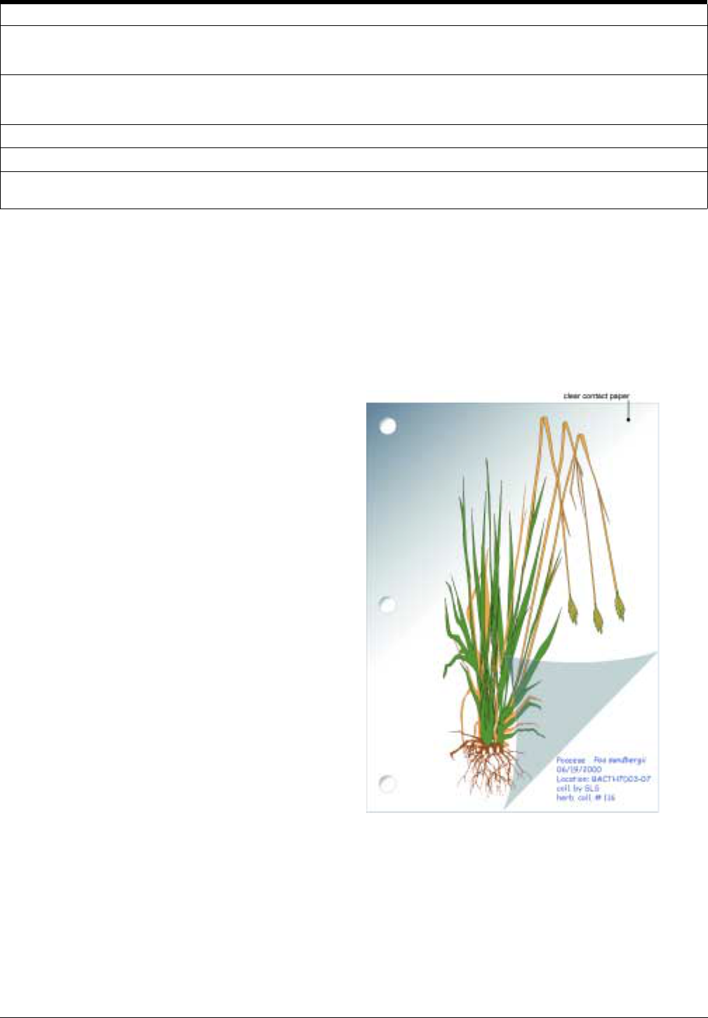
Date: Plot ID: Collected by: Coll. #

Latin Name:

Common Name:

Family:

Description: ann/bien/per Life form:

flr. color: other:

fruit type:

ht.: Habitat:

Topo Quad: Assoc. spp.:

Location (

UTM, lat/long): Elev.: Slope: Aspect:

Comments:

Figure 42. Voucher specimen data collection form.

PRESSING AND DRYING

Press your collected specimens as soon as possible;

fresh samples are far more flexible and will allow you

to position them well on the page. Keeping a standard

plant press in your vehicle will allow you to press spec-

imens promptly.

Use of the Press

It is important to place the end pieces of the press

right-side-up or the pressure from securing the straps

may break the wooden strips. Between the end pieces,

create sets of layers as follows: a sheet of corrugated

cardboard, then a sheet of blotter paper, then several

pages of newspaper, then another sheet of blotter

paper and another sheet of corrugated cardboard.

Place each specimen inside the folds of the newspaper.

The tabloid-size pages of weekly and monthly news-

print publications (university newspapers, entertain-

ment circulars, etc.) are often just the right size for

standard presses.

As each specimen is pressed, note on the top side of

the newspaper the collection number, plant name and

any other information needed to correlate the speci-

men with the field notebook entry. Print the species

name on the top side of each sheet so you do not have

to open the sheets to see what is inside.

Face each sheet of newspaper in the same direction

relative to the top side of the specimen and the fold.

The samples will require less handling this way. Indi-

cate the top side of the press and always open it

right-side-up. Never turn press sheets like pages in a

book; pieces will surely fall out with each turning.

Instead, open the press, carefully lift each sheet, face

up and with the open edge held slightly higher than the

folded end so loose material will not escape, and place

it aside.

Arrangement of Specimens on the Page

Size

Do not allow plant material to extend beyond the press

edges; this will allow your specimens to be damaged

when they are dry and fragile. Instead, arrange large

specimens to fit in the press (see Figure 43).

Figure 43. Pressing an oversized specimen.

(Shown mounted in an 8.5 × 11” field book.)

Trimming the specimen

It may be necessary to trim off some leaves or other

vegetative material to make a useful, uncluttered speci-

men. Do this carefully and with forethought; leaf posi-

tion is often an important feature. If you do remove a

leaf, leave part of the petiole to show the leaf position.

Never remove the petiole base and stem attachment or

Appendix C n

nn

n Field Aids 195

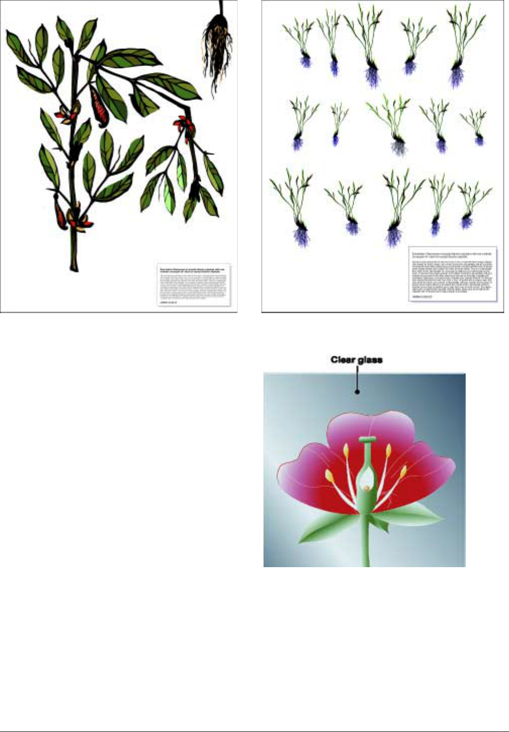
Figure 44. A nicely trimmed, tall specimen.

leaflets of a compound leaf, and don’t mistake a com-

pound leaf for a branch with individual leaves. Leave

twigs whole—do not split them (see Figure 44).

Arrangement

Once pressed, a single plant may not be rearranged, so

arrange it artfully at the first pressing. Of course, multi-

ple plants to be included on a single herbarium sheet

may be rearranged around each other upon mounting

(see Figure 45). Note that specimens of turgid plants

may be more easily arranged if you first allow the sam-

ples to wilt slightly. You may use a small piece of glass

(such as from a picture frame) so you can see the criti-

cal structures as you press them.

Flowers

If the flowers are large enough (e.g., Mimulus or Viola

or larger, most composites) cut one or two open and

press them flat so the internal structures are visible

(you can use your thumb to press open a flower, then

pop it into the press, or press it under a small piece of

glass). This is especially important in working with the

Polemoniaceae and monocots. Floral structures of the

composites are very important in identification, espe-

cially the phyllaries (bracts). Always include whole

flowers as well (see Figure 46).

Figure 45. Arranging small plants on a single herbarium

sheet.

Figure 46. Pressing flowers in an open state.

Vegetative parts

Press these in such a way that all important, or poten-

tially important, diagnostic features are visible. Show

both dorsal and ventral leaf surfaces, flatten out

stipules, expose the nodes, and clean off the roots. If

you must fold a leaf, keep the base and apex exposed

(see Figure 47).

Fire Monitoring Handbook 196

Figure 47. The right and wrong ways to press a large leaf.

Loose fruits, seeds and other structures

Store loose structures in envelopes or packets made

out of newspaper. Make sure each packet is labeled.

Drying and Freezing

Back in the office or lab, finish keying the specimens

and compare them with any existing herbarium speci-

mens. Once your identification is complete, you are

ready to mount specimens. To prevent molding, first

dry the specimens thoroughly. To prevent the intro-

duction of insects to the collection, treat your speci-

mens before moving them into an herbarium.

Commonly such treatment is done by wrapping plants

in plastic and freezing them for a week or two. If you

mount specimens in the office, freeze them after

mounting. If you mount specimens in the herbarium,

freeze them before mounting.

MOUNTING, LABELING AND STORING

Choosing a Voucher Style

The best system for vouchering the specimens col-

lected on monitoring plots includes the preparation of

a set of official herbarium sheets to be accessioned

into the park collection, and the concurrent prepara-

tion of a set of smaller sheets for inclusion in a binder

that can be easily and quickly accessed by monitors and

taken into the field when necessary. Alternatively, you

can establish a “working herbarium” for more casual

use. See the section on “Storing” below for a detailed

discussion of the various options.

Herbarium Specimens

Properly prepared and stored herbarium specimens

have an almost indefinite life span. Use only archival

quality mounting materials (acid-free mounting and

label paper, glue, etc.), which will not deteriorate over

time. The collection curator may have these on hand,

or they can be purchased from standard curatorial

sources. Never mount specimens with ordinary tape,

staples or contact paper.

Create an aesthetically pleasing herbarium specimen by

carefully considering the placement of plant material

on the sheet.

Labeling

The herbarium curator may require the use of a stan-

dard labeling form. In any case, the following informa-

tion should be included on the label as shown in

Figure 48:

• Genus, specific epithet and author

• Family name

• Exact location (including county, topographic quad

name, township, range, section, elevation, burn unit,

place name, access road, approximate mileage, etc.)

• Habitat description (e.g., wet meadow, oak wood-

land, dry coniferous forest understory, dry pinyon-

juniper woodland)

• Associated species (especially the most common or

dominant)

• Collector’s name

• Collection date

REDWOOD NATIONAL AND STATE PARKS

HUMBOLDT AND DEL NORTE COUNTIES, CALIFORNIA

HERBARIUM COLLECTION

Latin Name: Agrostis capillaris L.

Family: Poaceae

Cat. No.: 4149

Acc. No.: 00153

Locality: FQUGA4D09–04, Dolason Prairie,

see FMH-5 for further information

Elev.: 2320'

Habitat: Coastal Prairie

Assoc. Spp.: Arrhenatherum elatius, Elymus glaucus, Danthonia californica,

Trifolium dubium, Rumex acetosella, Anthoxanthum aristatum.

Collected by: T. LaBanca and D. Brown Date: 6/12/01

Adapted from USDI NPS form 10-512 (USDI NPS 2001c).

Figure 48. Example of an herbarium label.

Storing

Herbarium specimens should be stored according to

NPS curatorial guidelines. If you choose to set up an

additional, more accessible “working herbarium,” pur-

chase an herbarium cabinet and specimen folders for

this use, and keep your specimens under the best cli-

matic conditions possible with regard to humidity and

temperature. Herbarium Supply recommends 20–25°C

and 40–60% (or lower) RH. Consult with your park

curator for more information.

Appendix C n

nn

n Field Aids 197

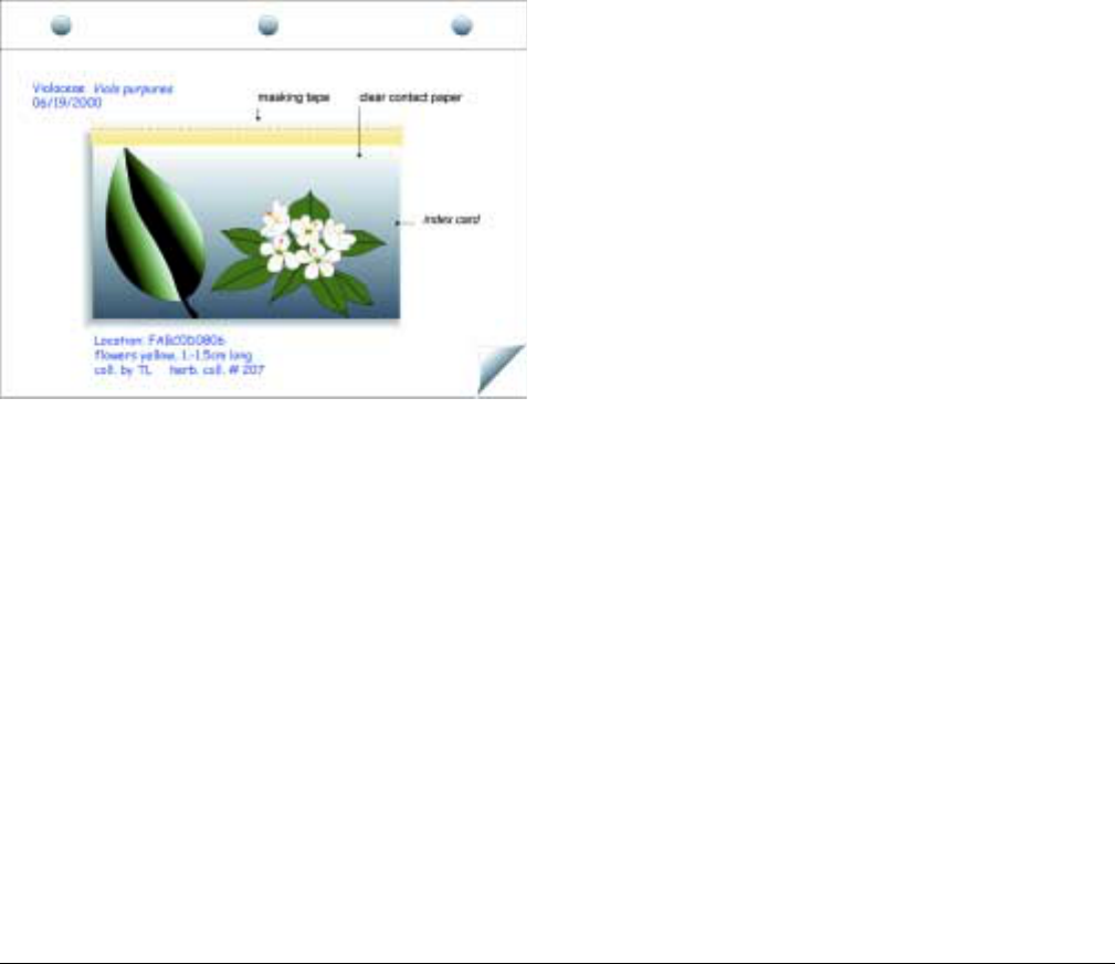
Field Specimen Books

Your field specimen books will be an invaluable

resource in the field and the office. When preparing

the herbarium specimens, reserve some good exam-

ples of each specimen for the field book. Labeling in a

field book is less formal than that of an herbarium, and

can be abbreviated (as long as there is a corresponding

herbarium specimen to which you can refer). At a min-

imum it must include the plant name (botanical and

common, if desired) and family, the plot near which it

was found, the collection date, the initials of the collec-

tor, and characteristics important in distinguishing

between similar species (length of petals, number of

leaflets, size of auricles, etc.). Make sure to also include

the number of the herbarium specimen to which it

corresponds. Arrange the pages by family, then genus

and species. You can create separate books for differ-

ent habitats as the collection grows. Compilation pages

can be included, comparing easily confused species

such as some ephemerals, or conifer seedlings.

paper. Taping the specimens directly to paper is not

recommended as the specimens tend to get easily

damaged with use. If the book is for office use only,

you can use plastic sheet protectors; however, these

may not be protective enough if the books are to be

used in the field (see Figure 43, page 195).

Figure 49. Example of a page from a field specimen book.

Two common styles of field specimen books are:

• 5 × 7 in three-ring binders: Label an index card

with the appropriate information. Encase the speci-

men between two layers of 3–4 in-wide packing tape

or clear contact paper so that both sides of the spec-

imen are visible. If the specimen is too big, include

just the critical features, or split the specimen onto

two cards. Then tape the encased specimen onto the

index card at the top so that it can be flipped up for

viewing the underside of the specimen (see

Figure 49).

• 8½ × 11 in three-ring binders: Mount specimens

to labeled sheets of acid-free paper with clear con-

tact paper. The contact paper tends to separate; take

care that the contact paper is securely adhered to the

Fire Monitoring Handbook 198

Identifying Dead & Dormant Plants

Vegetation monitoring and sampling is best done dur-

ing the “height of the bloom,” when most plants are

flowering and thus most easily identified. In areas with

a bimodal rainfall pattern, or otherwise weak seasonal-

ity (such as the southwest or the southeast), it may be

best to regularly sample more than once per cycle. This

allows you to catch entire suites of plants that you may

otherwise miss.

Regardless, you will invariably encounter a few early

bloomers that have already gone to seed, or some late

blooming perennials that are still dormant. With care-

ful observation and a few additional resources you can

still identify dead and dormant plants.

Identifying Species Using Only

Vegetative Characters

Consider any determination that you make using only

vegetative characters as tentative until you can make a

comparison with a flowering specimen.

RESOURCES

Always carry a species list and data sheets from previ-

ous visits or similar locations. In addition, be familiar

with locally represented plant families and their charac-

teristics. Here are some resources you will want to use:

• A species list for the area of concern and data sheets

from previous visits, if available

• Your favorite flora

• Your field herbarium

• A locally oriented vegetative plant identification

guide if available. Note: There are numerous vegeta-

tive keys to plant species and their seedlings (e.g.,

trees, shrubs, grasses, weeds, etc.) available for many

locations (see the bibliography in Appendix G, page

240)

OBSERVATIONS

The key to good science is good observation. One of

the best techniques for identifying a cured, dehisced,

or dormant plant is to gain familiarity with the plant

during its flowering or fruiting stage. Go out in the

field earlier than usual in the season and look around

for the early bloomers, then go out again for late or

off-season bloomers.

Another technique is careful observation of the clues

at hand. Spend some time with the plant in question,

and really look at it. Carefully examine the following

characteristics (refer to a botanical glossary for defini-

tions of these terms) and take notes on any available

field clues:

• Leaves, stipules and leaf scars: arrangement

(alternate, basal, opposite, whorled), attachment

(clasping, petiolate, sessile), color, form (compound,

simple, pinnate, needle-like), margin (e.g., entire,

lobed, serrate), odor, shape (e.g., broad, narrow),

size, stipules (presence and characteristics), texture

(e.g., durability, smoothness, pubescence (including

type, e.g., glandular, stellate, scales))

• Buds: arrangement (e.g., appressed, clustered),

color, scales (i.e, arrangement, number, shape, tex-

ture), size, shape, texture (e.g., smooth, scaly, pubes-

cent (including type, e.g., glandular, stellate, scales)),

type (leaf vs. flower)

• Stems and Twigs: branching (e.g., extensive or lim-

ited, form), color, flexibility, texture (e.g., durability,

smoothness, pubescence (including type, e.g., glan-

dular, stellate, scales)), thorns (number, length,

shape), odor, pith (color, composition), amount of

woody tissue

• Flowers: if there is any evidence of flowers, you may

be able to determine: arrangement (e.g., catkin, pani-

cle, cyme, umbel), color, dehiscence, fragrance, loca-

tion (terminal, lateral, new or old wood), filaments

(fused, free), stamens (presence, number), number of

stigmas/styles/pistils, ovary (superior, inferior or

partly), sepals (characteristics, e.g., length, number,

texture), presence of a floral bracts, presence of a

hypanthium, size, type (e.g., radial, bilateral)

• Fruit (look on plant and beneath it): color, location

(e.g., old or new wood, terminal or lateral), number

of carpels, placenta (axile, parietal, free-central), seed

characteristics (e.g., attachment, number), shape (e.g.,

flat, round, winged), texture (e.g., dry, fleshy), type of

fruit (e.g., achene, berry, capsule, follicle, legume,

utricle)

• Bark: color, texture (e.g., checkered, flaky, lined,

smoothness, lenticles, pubescence (including type,

e.g., glandular, stellate, scales)), thickness

• Form: ascending, columnar, conical, decumbent,

erect, globular, oval, prostrate, spreading, vase-like,

or weeping

• Sap: color, odor, texture

Appendix C n

nn

n Field Aids 199

• Habit: annual, biennial, perennial, vascular, non-vas-

cular, aquatic, terrestrial, parasitic, fern, shrub, tree,

vine, etc.

•Height

• Underground parts: branching, color, flexibility,

texture, type (e.g., bulb, stolons, rhizomes)

• Habitat: microclimate where it grew (e.g., dry, open

areas, crevices, moist clay, rocky)

Some families or genera have elements that are very

characteristic, even in the dried state; for example,

composites have receptacles, lilies have woody pods,

and umbels have grooved seeds and feathery inflores-

cences. You may also want to try smelling the plant to

see if it is familiar.

If you find that you are somewhat certain as to the

identification of the species at hand, compare your

specimen with previously identified specimens in a

herbarium or voucher collection. Compare the leaves,

stems, fruits, and other parts to identified specimens.

Note: Don’t take your specimen into the herbarium

without following the herbarium’s procedures for kill-

ing pests (usually, freezing). However, if you can’t iden-

tify your specimen, make a voucher, note its exact

location, and then visit it again when it is blooming.

Fire Monitoring Handbook 200

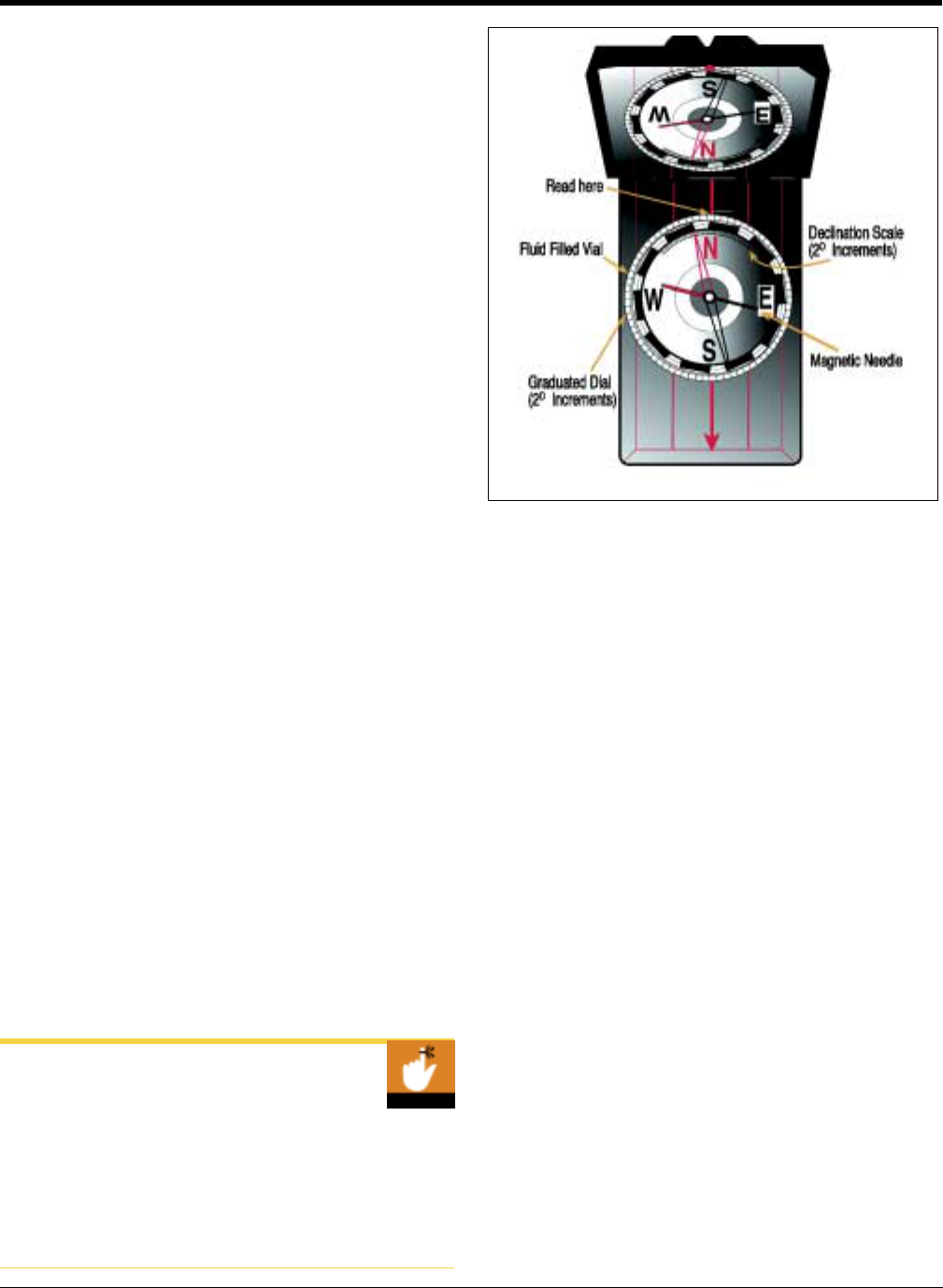
Navigation Aids

As field personnel, monitors must be able to navigate

over open terrain, determine distances traveled and

plot transect locations on a map. The following sec-

tions discuss the correct use of two of the basic tools

used by monitors in the field—a compass and a cli-

nometer—as well as some basic mapping techniques

for locating and mapping transect locations in the

field.

COMPASS

The compass is probably the instrument most fre-

quently used by field personnel. Accurate compass

bearings are essential for navigating over open terrain

and for finding and mapping plot locations.

Parts of a Compass

A multitude of compass models exist with different

features; however, all compasses have at minimum the

following:

Magnetic needle—The magnetic needle, drawn by

the pull of the magnetic north pole, always points to

magnetic north. The north end of the needle is usually

marked by an arrow, or painted red.

Revolving 360° dial—The dial is marked with the

cardinal points, N, E, S, W and is graduated into

degrees. Within the dial is a transparent plate with par-

allel orienting lines and an orienting arrow.

Transparent base plate—Has a line of travel arrow

and ruled edges.

Setting a Bearing

If you know the bearing in degrees (and your declina-

tion, see page 202) from your current position to an

object, turn the dial until the degree is aligned with the

index point and line of travel arrow. In Figure 50, the

bearing is set at 356°.

Obtaining Accurate Compass

Bearings

Always hold the compass level, so the magnetic needle

can swing freely. Hold the compass away from mag-

netic objects such as rebar, watches, mechanical pen-

cils, cameras, and belt buckles that can draw the

magnetic needle off line.

Figure 50. Graphic of a compass.

Taking a Bearing

• Aim the line of travel arrow on the compass towards

the object.

• Turn the revolving dial until the magnetic needle is

aligned within the orienting arrow in the compass

dial.

• Read the bearing on the compass dial at the index

point.

Facing a Bearing (Direction of Travel)

Hold compass with the base plate level and line of

travel arrow pointing forward. Turn your body with

the compass until the red north end of the magnetic

needle point is aligned within the orienting arrow in

the compass dial. You are now facing in the direction

of the bearing.

Walking a Bearing

Look straight ahead in the direction of travel. Choose a

landmark that lies in line with the direction of travel.

Walk to the landmark. Continue in this manner until

you reach your destination.

USING A COMPASS IN CONJUNCTION

WITH A MAP

You may use a compass in conjunction with a map in

either of two ways:

Appendix C n

nn

n Field Aids 201

• Determine a bearing from a map and then travel that

direction in the field (map to terrain), or

• Take a bearing in the field and plot that bearing on a

map (terrain to map).

Whenever combining compass (field) bearings with

map (true) bearings, you must account for declination.

Declination

Declination is the degree of difference between true

north and magnetic north. True north is where all lines

of longitude meet on a map. Magnetic north is the

location of the world’s magnetic region (in the upper

Hudson Bay region of Canada).

Declination is east or west, depending upon where

magnetic north lies in relation to your position. If mag-

netic north lies to the east of your position, declination

is east. If magnetic north lies to the west of your posi-

tion, declination is west. In North America, zero decli-

nation runs roughly from west of Hudson Bay down

along Lake Michigan to the gulf in western Florida.

Declination diagrams are located in the bottom margin

of USGS topographic maps. Keep in mind that decli-

nation changes slightly over time as magnetic north

moves slowly west; therefore, the current declination

in your area may be slightly different than the declina-

tion at the time the map was printed. Declination maps

are re-mapped every five years by the USGS; the most

recent declination map is for 1995 (see Figure 51).

On some maps the annual rate of change may be

printed and thus you can calculate the current declina-

tion. USGS also produces a Magnetic Declination Map

of the United States. This map shows the rate of

change throughout the US so that the current declina-

tion in any area can be calculated. You may also obtain

the current declination in your area from your county

surveyor.

If you need to be more precise, try using a geomag-

netic calculator (e.g., NOAA 2000) that will calculate

the declination for any year (1900–2005) given the lati-

tude/longitude or UTM coordinates.

Setting declination on your compass

Some compass models have a declination adjustment

screw. The set screw key is usually attached to a nylon

cord that hangs from the compass. Using the key, turn

the set screw to the appropriate declination. Once you

have set the proper declination you do not need to

change it until you move to a different area. If you

Figure 51. Map showing declination in North America.

East of the zero line, declination is “west.” West of the zero line,

declination is “east.”

move to a new area, remember to reset the declination

on your compass. If you do not have a compass with a

declination adjustment screw, you must add or subtract

declination to determine the correct bearing. Whether

you add or subtract declination depends on whether

you are working from map to terrain or terrain to map.

Map to terrain

If you have determined a bearing between two posi-

tions from a map, and you are going to walk the bear-

ing, you must convert that bearing to a magnetic

bearing. The rules for converting from map to field

bearings are as follows:

• For declination west, turn dial west (add number of

degrees of declination)

• For declination east, turn dial east (subtract number

of degrees of declination)

Terrain to map

If you have taken a field bearing and want to plot the

position on a map, you must convert the bearing from

a magnetic bearing to a map (true) bearing. The rules

are simply the reverse of the map to terrain rules:

• For declination west, turn dial east (subtract)

• For declination east, turn dial west (add)

CLINOMETER

A second important field tool is a clinometer, which

measures slope in degrees and/or percent. Slope is one

of the most important topographic influences on fire

behavior. In addition, recording the slope along the

plot azimuth is another aid in defining (and thus relo-

cating) plots.

Fire Monitoring Handbook 202

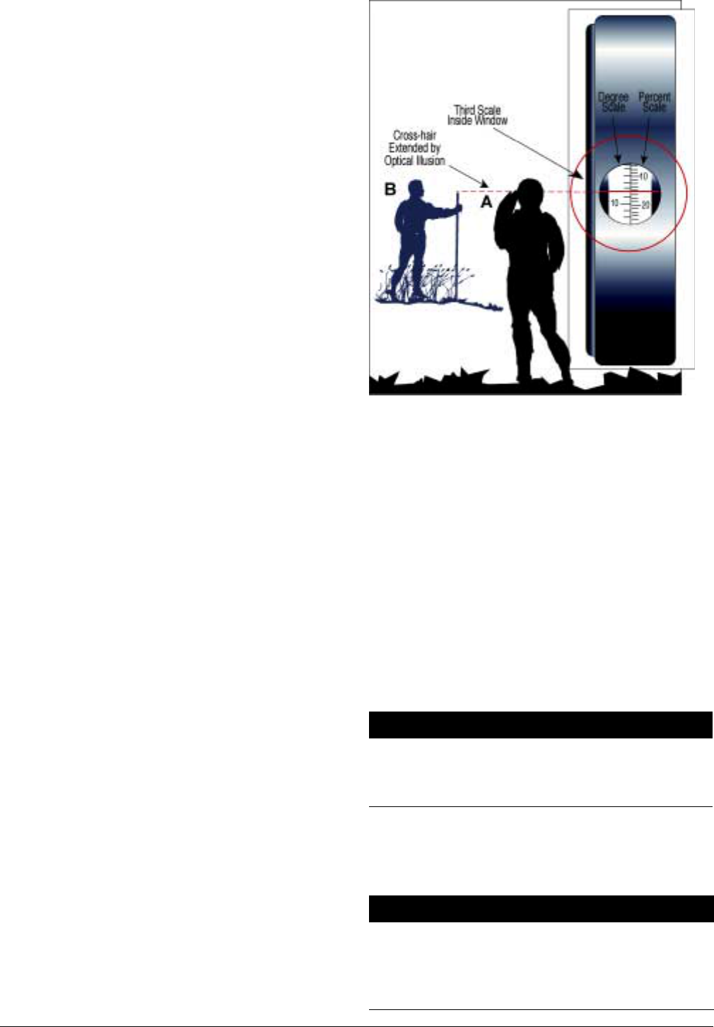
Measuring Slope Using a Clinometer

The model of clinometer most commonly used in fire

effects monitoring has both a degree scale and a per-

cent scale. When you look through the lens, you will

see the percent slope scale on the right side and the

degree scale on the left (see Figure 52).

Slope can be measured in degrees or as a percent. For

our purposes, measurements are made in percent slope

rather than in degrees; degrees slope is not used in this

handbook. Percent slope measures the degree of

incline over a horizontal distance; a +1% slope indi-

cates the rise is very gradual over a given distance. A

+60% slope indicates the rise is very rapid over a given

distance.

The degree scale gives the angle of slope in degrees

from the horizontal plane at eye level. The percent

scale measures the height of the point of sight from

the same horizontal eye level and expresses it as a per-

cent of the horizontal distance (i.e., % slope); percent

slope is used throughout this handbook. For a conver-

sion table between degrees slope and percent slope,

see Table 34, page 211.

To use a clinometer:

• Hold the clinometer so that the round side-window

faces to the left.

• Hold the clinometer up to your right eye but keep

both eyes open (you can hold the instrument up to

your left eye, if that is more comfortable).

• Aim the clinometer in the direction of the slope you

want to measure.

• Fix the hair line of the clinometer on an object in

your line of sight and at the same height as your

eye level, a rangepole may be useful.

• Look into the viewing case, and read where the hair

line intersects the percent scale (on the right).

DETERMINING DISTANCES IN THE FIELD

Distances along the ground can be measured by vari-

ous means. You can measure distances along a road in

a vehicle with an odometer. In the field you can use a

meter tape, though over long distances this method is

often impractical. Pacing is a common means of mea-

suring distance in the field. By knowing the length of

your pace you can measure the distance over ground

simply by walking. A pace is defined as the distance

between the heel of one foot and the heel of the same

foot in the next stride. Therefore, one pace equals two

steps—one step of each leg.

Figure 52. Graphic of a clinometer.

Note: The rangepole at B is the same height as the viewer's (A)

eye level. Also note that you can find clinometers with percent on

either the right or left side; percent being the larger number.

Determining Your Pace on Level Ground

• On level ground, lay out a course of known distance

(e.g., 50 m or 1 chain).

• Walk the length of the course counting each pace

(two steps). Take the first step with your left foot,

then count each time your right foot touches the

ground.

• Repeat the process several times to obtain an aver-

age number of paces per length.

• Divide the number of paces into the measured dis-

tance to arrive at the length of your pace.

Example:

50 m/32 pace = 1.6 m/pace

66 ft/20 pace = 3.3 ft/pace

To determine the distance you have paced in the field,

multiply the number of paces by your distance per

pace.

Example:

The distance between the reference feature and 0P

is 30 paces. Your pace distance is 1.6 m.

30 paces × 1.6 m/p = 48 m

Appendix C n

nn

n Field Aids 203

Determining Your Pace on Sloping Ground

Walking on a slope, either uphill or downhill, your

paces will be shorter; consequently you will take more

paces to cover the same distance on a slope as on level

ground. To determine your pace on sloping ground:

• Lay out a course of the same distance used on level

ground with moderately steep slope.

• Walk upward on this course, counting the number of

paces as before.

• Divide the total distance by the total number of

paces.

• This is the length of one pace on a slope.

Example:

On level ground: 50 m = 32 paces = 1.60 m/pace

On sloping ground: 50 m = 40 paces = 1.25 m/

pace

Walk the course several times both uphill and downhill

until you have an average length of a pace on sloping

ground. Your upslope pace may be different than your

downslope pace.

SOME BASIC MAP TECHNIQUES

Working with Scale

You will inevitably use maps with many different scales

during your monitoring work. A table of scales and

equivalents is located on page 212 (Table 35). If you

enlarge or reduce a map, the scale of the map will

change and you must determine the new scale. Scale

on a map is determined by the formula:

Map Distance MD)(

Scale = -------------------------------------------------------

Ground Distance GD)(

Map distance equals the distance measured between

two points on a map. Ground distance equals the dis-

tance on the ground between the same two points.

To determine the new scale of a map that was enlarged

or reduced, follow these steps:

• On the original map of known scale, measure the

map distance between two points that are separated

horizontally and two points that are separated verti-

cally. (The reason to measure two distances is that

copy machines are not precision instruments and

may skew the map.)

• Compare the distances to the original map scale to

determine the four ground distances.

• On the enlarged (or reduced) map, measure the dis-

tances between the same four points. (Although the

map distance has changed, the ground distances

between the four points are still the same.)

• Calculate the scale of the enlarged (or reduced) map

with the scale formula, using each of the four dis-

tances.

• Average all four scales, and use this for determining

ground distances on the enlarged (or reduced) map.

Example:

You calculate the scale of a map from an original map

at the scale of 1:24,000. On the original map, you

measure two separate horizontal distances, 5.6 and

11.1 cm, and two vertical distances 4.15 and 6.5 cm.

For a 1:24,000 map, 1 cm = 240 m (see Table 35,

page 212), so the corresponding ground distances are

1,344, 2,644, 996, and 1,560 m respectively.

Using the enlarged map, now measure the same four

distances. Using the first map distance-ground dis-

tance combination, we get the following scale:

MD 13.2 cm 1 cm

Scale = --------- = ------------------ = ---------------------

GD 1344 m 101.82 m

Continuing on for the three remaining distances, the

four resulting scales would be 1:10,182; 1:10,129;

1:10,163; and 1:10,163. Taking the average of these

four numbers, the scale of the enlarged map is deter-

mined to be 1 cm = 101.59 m, or 1:10,159.

Determining the Direction and Distance Between

Two Map Points

You will have to determine the direction and distance

between two map points when you use a map to get to

your Plot Location Points (PLP).

Determining the direction between two map points

To determine the direction between two points on a

map, follow these steps:

• Draw a line connecting the two points (A B).

• Place your compass with the edge of the base plate

along the line.

• Orient the compass with the line of travel arrow

pointing towards point B.

• Turn the revolving dial of the compass until the ori-

enting lines within the compass dial are parallel with

the north-south meridian lines on the map, and the

North (N) arrow points to north on the map.

Fire Monitoring Handbook 204

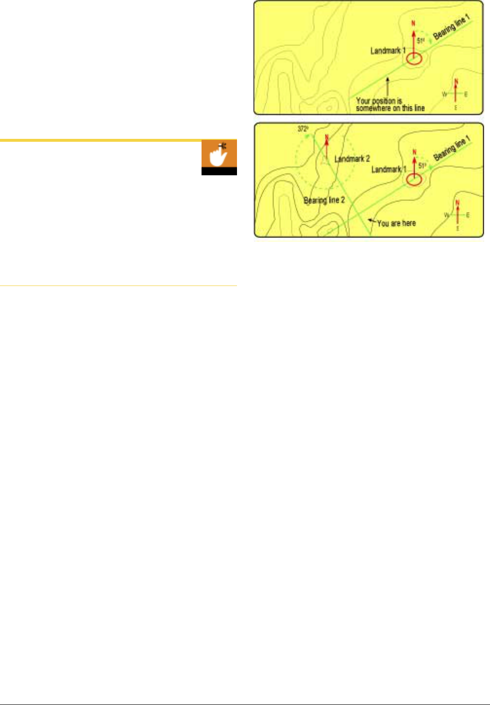
• Read the bearing at the index point on the compass.

Note: The direction of the magnetic needle is irrele-

vant in this procedure.

If you are going to set a field bearing using this map

bearing, remember to add or subtract the declina-

tion according to the rules in the previous section

(page 202). If your compass has the declination set,

you do not need to make any adjustments.

Map Direction

You can use a protractor in place of a compass in this

procedure. Simply place the black etched line on the

center of the protractor cross bar on point A and make

sure that 0° or 360° points towards North on the map.

Read the number of degrees where the line drawn

between points A and B intersects the protractor’s

outer edge.

Determining the distance between two map points

• Align the edge of a piece of paper with the line

drawn between the two points.

• Make a mark on the paper at points A and B.

• Hold the paper against the scale on the bottom of

the map.

• Measure the distance against the map scale.

Determining a Plot Location in the Field

You can determine plot locations with either of two

instruments: a compass or a Global Positioning Sys-

tem (GPS) unit. All plot locations, especially the origin

(forest plots), or 0P (grassland and brush plots),

should be defined at some time with a GPS unit so

they can be included in your park GIS database.

You can use a compass to plot a location on a topo-

graphic map in the field using a method known as

resection. You must first identify two landmarks (e.g.,

buildings, lakes, ridgetops) on the terrain that you can

pinpoint on a map. Once you have identified your two

landmarks, follow these steps (see Figure 53):

• Take a field bearing from your location to one of the

landmarks, adjusting for declination if necessary.

• Place compass on the map with one edge of the base

plate intersecting the landmark point.

Figure 53. Illustration of the resection method to determine

a plot location in the field.

• Keeping the compass edge against this point, turn

the entire compass, not the dial, until the compass

orienting lines are parallel with the north-south

meridian lines on the map and the N points to the

direction of north on the map.

• Draw a line along the edge of the compass intersect-

ing the point; your location lies somewhere along

this line.

• Repeat the process with the second point to draw a

second line on the map. The intersection of the two

lines is your location.

Determining Plot Location Using UTM

Coordinates on a USGS Topographic Map

Locate the UTM grid line markings along the edge of a

USGS topographic map. You can purchase clear Mylar

overlays that indicate the increments between the map

lines. To use them, simply find the closest UTM mark-

ings on the map edge, follow those out to the plot (or

other location) you wish to map, place the overlay on

the map and count the increments.

GLOBAL POSITIONING SYSTEM

INFORMATION

Many NPS units have access to PLGR units, a type of

GPS unit. This summary is intended to provide a quick

reference for some basic tasks that are commonly per-

formed in fire effects monitoring work (for further

information, see USDI NPS 1997).

Appendix C n

nn

n Field Aids 205

This section is not intended to replace training on the

use of PLGR or any other GPS units. In general, enter

and change information on the PLGR by using the

right and left arrow keys to highlight a field (make it

blink), then use the up and down arrow button to

select the field.

Displaying Your Current UTM Coordinate

Position

Turn on the PLGR. The position screen will appear. In

the upper right corner of the screen the word OLD

will appear indicating that the information displayed

on the rest of the screen is from a previous or old loca-

tion. After the PLGR obtains signals from four or

five satellites the word OLD is replaced by the

PDOP (see Glossary), which is the amount of error

for the displayed position (this calculation might

take a few minutes). Enter this error information

into the FMH-5. If the level of error is acceptable for

your GIS specialist, store your location as a waypoint

(see below).

For the best accuracy, go to MENU, then SETUP and

change the SETUP MODE to AVG. This will allow

the PLGR to average points together to give you a

more accurate reading of your location. The number

of points averaged is shown in the upper part of the

screen (>

180 points is desirable). It is important not to

move the location of the PLGR while in averaging

mode, as this prevents the unit from obtaining an

accurate reading.

Store a Position as an Individual Point Called a

Waypoint

To store the UTM coordinates of your current posi-

tion as a waypoint, press the MARK button twice. The

position will be stored as WP001, WP002, WP003, etc.

It is useful to include a small notebook with the PLGR

for tracking waypoint numbers to assist with their defi-

nition at a later date, e.g., “WP01 = Oak Flat trail-

head.”

To clear a waypoint, press WP, select CLEAR, type in

the waypoints you wish to delete, then select ACTI-

VATE/CONFIRM.

Navigate to a Known Waypoint from Your Current

Location

To navigate to a known waypoint, press NAV, and then

choose “2D Fast and DIRECT” on the top line. On

the second line, press NUMLOCK to activate the

numeric keypad (“N” will be displayed in the lower

right corner instead of “P”) and enter the number of

the desired waypoint, or simply scroll to the desired

waypoint number. Page down to the next screen,

which lists the selected waypoint, and the distance

(RNG) and direction (AZ) you should travel from your

current location.

Obtain Distance and Direction Between Two

Waypoints

Use this feature to calculate the distance and azimuth

between two remote locations once they have been

marked as waypoints. You can then transfer this infor-

mation to your plot location maps, e.g., distance from

reference point to a plot point (Ref–0P), or use it to

navigate from plot to plot without returning to a start-

ing point.

Press the WP key, then select DIST. The next screen

will allow you enter two waypoints; it will then display

the range (distance) and azimuth from the first way-

point to the second waypoint.

Geodetic Datums

The reference systems that define Geodetic datums

describe the earth’s size and shape. Various datums are

used by different countries and agencies, and the use of

the wrong datum can result in tremendous position

errors of hundreds of meters. GPS units use WGS84

for all data capture, but can output data in a variety of

datums. Select the datum that matches the GIS data of

your park unit, or tell your GIS specialist which datum

you used so the data can be converted. The following

datums are used in the US and its territories:

Abbreviation Full Title

NAD27 North American Datum-1927, Continental US

(Conus)

NAD83 North American Datum-1983, Continental US

(Conus)

NAD83 North American Datum-1983, Hawaii

(Hawaii)

WGS84 World Geodetic System-1984

OHD26 Old Hawaiian Datum (Mean)-1926

ASD62 American Samoa-1962

GD63 Guam Datum-1963

Fire Monitoring Handbook 206

3

Basic Photography Guidelines

When photographing outdoors, you should strive to

strike a balance between the quality of the film image,

ambient light levels and depth of field (how much of

the view is in focus). The three ways to control these

factors are 1) film speed, 2) shutter speed and 3) aper-

ture size (how wide the shutter opens).

The following procedure may be followed to obtain

high quality photos:

• Film Speed: Use the slowest film possible while

still maximizing the depth-of-field (64 or 200 ASA

Kodachrome, 100–400 ASA Fujichrome or

Ektachrome).

Film speed should be carefully selected to repre-

sent the slowest speed (lowest ASA) acceptable for

the ambient light conditions. For example, photog-

raphy in a dark forest understory requires a faster

speed such as 200 ASA or even 400 ASA, but in a

bright, open prairie 64 ASA may be the best

choice. In this case, the faster speed films (higher

ASA) would also work in the prairie, but will not

produce as sharp an image as the slower speed

film.

It is advisable to purchase a range of film speeds

reflective of the lighting conditions likely to be

encountered at your unit, and to switch film (mid-

roll if necessary) when drastic changes in lighting

occur (such as a switch from dark forest plots to

light brush plots). You may want to consider hav-

ing a second camera to help manage films of dif-

ferent speeds.

Remember that although higher speed film can be

used in higher light conditions, to avoid blurry

photos do not use lower speed film in lower light

conditions. If you desire one all-purpose film

speed, choose 64 ASA for open areas and use 200

ASA for darker conditions.

• Exposure: Once you have selected the subject,

set the exposure, a combination of aperture (also

called f/stop) and shutter speed.

Try to obtain f/16 and still have a shutter speed of

1/60 second or faster if the camera is handheld

(slower speed is fine if the camera is mounted on a

monopod or tripod). If the light meter indicates

that more light is needed, then back off to f/12 or

f/8 (try to get the smallest aperture possible,

which is indicated by the highest number). The

light meter will indicate when an acceptable setting

has been reached. Be sure that the light meter

reading has not included any sky.

Keep your shutter speed as fast as possible to

avoid blurry photos. Under the same conditions, a

slower film speed will require a slower shutter

speed and a faster film speed will allow for a faster

shutter speed. If the camera is hand-held, the shut-

ter speed should be kept at or above 1/60 (one-

sixtieth of a second), although some very steady

hands can push this to 1/30. If a monopod or tri-

pod is used with a cable release, any shutter speed

will work.

• Depth of Field: Set the depth of field (the focus

mechanism on the lens) to include the farthest

object visible in the shot (usually infinity).

Aperture, or f-stop, dictates the depth-of-field (the

distance to which the photo will be in focus). For

plot photography it is usually desirable to have a

depth-of-field of infinity, with a corresponding f-

stop of f/11 or f/16 (or occasionally f/8, if the

view is not deep anyway, due to tall vegetation).

The aperture setting interacts with the shutter

speed; as the shutter speed increases, the aperture

must widen (indicated by a smaller number),

reducing the depth-of-field.

You are now ready to take the shot. Don’t change

the lens setting or focus, even if the view seems

out of focus; it will give an excellent, clear shot

with the entire field of view in focus if set from the

above instructions.

Note the nearest distance that will be in focus

(shown on the depth-of-field indicator).

• Set up the Shot: Look through the viewfinder

and place the bottom of the view at the nearest

distance that will be in focus.

Select an object in the center of the view that is

easy to find (e.g., the tape or rangepole) and center

the shot on it, using the “cross hairs” as a refer-

ence.

• Shoot: Be sure that the camera is level, and shoot.

Appendix C n

nn

n Field Aids 207

The following table (Table 32) demonstrates a few

examples of different environmental conditions, film

speeds, camera settings and the results you may expect.

Table 32. Results you may expect from different environmental conditions, film speeds, and camera settings.

Environmental Setting Film Speed Shutter

Speed

Aperture

Setting

Results

Open Prairie—Sunny Day

64 ASA

200 ASA

64 ASA

200 ASA

1/250

1/500

1/60

1/15

1/30

1/15

f/16

f/11

f/5.6

f/11

f/16

f/5.6

Highest quality, clear image

High quality, clear image

Light OK, but only the foreground is in focus

due to small aperture setting. Use higher

speed film to enable higher aperture.

Good depth of field, light OK, but blurry due to

slow shutter speed. Try changing the aperture

to 8, or using a monopod or tripod.

Good quality image

Don’t bother. Return earlier on another day

with better light conditions. Bring a monopod or

tripod. Consider higher speed film if conditions

are always very dark.

Open Prairie—Sunny Day

Shaded Woodland—

Sunny Day

Shaded Woodland—

Sunny Day

Dark Forest—Sunny Day

with Monopod or Tripod

Dark Forest—Cloudy Day,

Late Afternoon in Autumn

Fire Monitoring Handbook 208

3

Conversion Tables

Table 33. Conversion factors. Table 33. Conversion factors. (Continued)

Acres 0.4047 Hectare or sq. Grams 0.03527 Ounces

hectometer

Grams

2.205 × 10

-3

Pounds

Acres 43,560.0 Square feet

Hectares 2.471 Acres

Acres 4,446.86 Square meters

Acres

1.563 × 10

-3

Square miles

Hectares 107,600 Square feet

Hectares 10,000 Square meters

Centimeters

0.03281

Feet

Hours 0.041672 Days

Centimeters 0.3937 Inches

Hours

5.952 × 10

-3

Weeks

Centimeters 0.1 Decimeters

Inches 2.54 Centimeters

Centimeters

10

-5

Kilometers

Inches 0.0254 Meters

Centimeters 0.01 Meters

Inches

1.578 × 10

-5

Miles

Centimeters

6.214 × 10

-6

Miles

Inches 25.4 Millimeters

Centimeters 10.0 Millimeters

Inches/sec 5.0 Feet/min

Centimeters

0.01094

Yards

Inches/sec

1.2626 × 10

-3

Chains/hour

Chains 66.0 Feet

Inches

0.02778

Yards

Chains 792.0 Inches

Kilograms 1,000.0 Grams

Chains 20.12 Meters

Kilograms 2.205 Pounds

Chains/hour 3,600 Inches/sec

Kilograms

9.842 × 10

-4

Tons [Long]

Chains/hour 0.01833 Feet/sec

Circumference of 0.3183 DBH

Kilograms

1.102 × 10

-3

Tons [Short]

a tree

Kilograms/square 4.462 Tons [Short]/acre

Decimeter 0.1 Meters

meter

Degrees (Celsius) (1.8 C°) + 32° Degrees

Kilometers 100,000 Centimeters

(Fahrenheit)

Kilometers 3,281.0 Feet

Degrees (5.5 F°) - 32° Degrees (Celsius)

Kilometers 39370.0 Inches

(Fahrenheit)

Kilometers 1,000.0 Meters

DBH 3.1416 Circumference of

a tree

Kilometers 0.6214 Miles

Feet 0.01515 Chains

Kilometers 1,093.6 Yards

Feet 30.48 Centimeters

Kilometers/hour 27.78 Centimeters/sec

Feet

3.048 × 10

-4

Kilometers

Kilometers/hour 54.68 Feet/min

Feet 0.3048 Meters

Kilometers/hour 0.9113 Feet/sec

Feet 304.8 Millimeters

Kilometers/hour 16.67 Meters/min

Feet/sec 0.8333 Inches/sec

Kilometers/hour 0.278 Meters/sec

Feet/sec 54.54 Chains/hour

Kilometers/hour 0.6214 Miles/hour

Feet/sec 0.305 Meters/sec

Meters 100.0 Centimeters

Appendix C n

nn

n Field Aids 209

IF YOU HAVE MULTIPLY BY TO GET IF YOU HAVE MULTIPLY BY TO GET

Table 33. Conversion factors. (Continued)

IF YOU HAVE MULTIPLY BY TO GET IF YOU HAVE MULTIPLY BY TO GET

Meters 0.04971 Chains

Meters 3.281 Feet

Meters 39.37 Inches

Meters

1.0 × 10

-3

Kilometers

Meters

6.214 × 10

-4

Miles

Meters 1,000.0 Millimeters

Meters 1.094 Yards

Meters/sec 178.9 Chains/hour

Meters/sec 196.9 Feet/min

Meters/sec 3.281 Feet/sec

Meters/sec 3.6 Kilometers/hour

Meters/sec 0.06 Kilometers/min

Meters/sec 1.943 Knots

Meters/sec 2.237 Miles/hour

Miles

160,900

Centimeters

Miles 5,280.0 Feet

Miles

6.336 × 10

4

Inches

Miles 1.609 Kilometers

Miles 1,609.0 Meters

Miles 1,760.0 Yards

Miles/hour 44.7 Centimeters/sec

Miles/hour 88.0 Feet/min

Miles/hour 1.467 Feet/sec

Miles/hour 1.609 Kilometers/hour

Miles/hour 0.45 Meters/sec

Millimeters

3.281 × 10

-3

Feet

Millimeters 0.03937 Inches

Millimeters

1.0 × 10

-6

Kilometers

Millimeters

1.0 × 10

-3

Meters

Millimeters

6.214 × 10

-7

Miles

Millimeters

1.094 × 10

-3

Yards

Ounces 28.35 Grams

Ounces 0.0625 Pounds

Ounces

2.79 × 10

-5

Tons [Long]

Ounces

3.125 × 10

-5

Tons [Short]

Pounds 453.6 Grams

Pounds 0.4536 Kilograms

Pounds 16.0 Ounces

Pounds

5.0 × 10

-4

Tons [Short]

Pounds

4.464 × 10

-4

Tons [Long]

Slope (Degrees) see table below Slope (Percent)

Slope (Percent) see table below Slope (Degrees)

Square Feet

2.296 × 10

-5

Acres

Square Feet 0.0929 Square Meters

Square Feet

3.587 × 10

-8

Square Miles

Square Meters

2.471 × 10

-4

Acres

Square Miles 640.0 Acres

Square Miles

27.88 × 10

6

Square Feet

Tons [Long] 1,016.05 Kilograms

Tons [Long] 2,240.0 Pounds

Tons [Short]/Acre 0.2241 Kilograms/square

meter

Tons [Short] 907.2 Kilograms

Tons [Short] 2,000.0 Pounds

Tons (Metric) 1,000.0 Kilograms

Tons (Metric) 2,204.6 Pounds

Yards 91.44 Centimeters

Yards

9.144 × 10

-4

Kilometers

Yards 0.9144 Meters

Yards

5.682 × 10

-4

Miles

Yards 914.4 Millimeters

Fire Monitoring Handbook 210

Table 34. Slope Conversions (Between degrees and percent).

Degrees Percent

Slope

Degrees Percent

Slope

Degrees Percent

Slope

Degrees Percent

Slope

1 1.7 24 44.5 47 107.2 70 274.7

2 3.5 25 46.6 48 111.1 71 290.4

3 5.2 26 48.8 49 115.0 72 307.8

4 7.0 27 51.0 50 119.2 73 327.1

5 8.7 28 53.2 51 123.5 74 348.7

6 10.5 29 55.4 52 128.0 75 373.2

7 12.3 30 57.7 53 132.7 76 401.1

8 14.1 31 60.1 54 137.6 77 433.1

9 15.8 32 62.5 55 142.8 78 470.5

10 17.6 33 64.9 56 148.3 79 514.5

11 19.4 34 67.5 57 154.0 80 567.1

12 21.3 35 70.0 58 160.0 81 631.4

13 23.1 36 72.7 59 166.4 82 711.5

14 24.9 37 75.4 60 173.2 83 814.4

15 26.8 38 78.1 61 180.4 84 951.4

16 28.7 39 81.0 62 188.1 85 1143.0

17 30.6 40 83.9 63 196.3

86 1430.1

18 32.5 41 86.9 64 205.0 87 1908.1

19 34.4 42 90.0 65 214.5 88 2863.6

20 36.4 43 93.3 66 224.6 89 5729.0

21 38.4 44 96.6 67 235.6 90 ∝

22 40.4 45 100.0 68 247.5

23 42.4 46 103.6 69 260.5

% Slope = 100 × Tan [Slope] = 100 × Vertical Rise/Horizontal Distance

Appendix C n

nn

n Field Aids 211

Table 35. Map scales and their equivalents in feet, meters, Table 35. Map scales and their equivalents in feet, meters,

and acres. and acres. (Continued)

Scale (1"

on a map=)

Feet per

Inch

Meters per

Inch

Acres per

Sq. Inch

Scale (1"

on a map=)

Feet per

Inch

Meters per

Inch

Acres per

Sq. Inch

1:500 41.67 12.70 0.04 1:20,400 1,700.00 518.16 66.35

1:600 50.00 15.24 0.06 1:21,120 1,760.00 536.45 71.11

1:1,000 83.33 25.40 0.16 1:21,600 1,800.00 548.64 74.38

1:1,200 100.00 30.48 0.23 1:22,800 1,900.00 579.12 82.87

1:1,500 125.00 38.10 0.36 1:24,000 2,000.00 609.60 91.83

1:2,000 166.67 50.80 0.64 1:25,000 2,083.33 635.00 99.64

1:2,400 200.00 60.96 0.92 1:31,680 2,640.00 804.67 160.00

1:2,500 208.33 63.50 1.00 1:33,333 2,777.78 846.68 177.14

1:3,000 250.00 76.20 1.43 1:48,000 4,000.00 1,219.20 367.31

1:3,600 300.00 91.44 2.07 1:50,000 4,166.67 1,270.03 398.56

1:4,000 333.33 101.60 2.55 1:62,500 5,208.33 1,587.50 622.74

1:4,800 400.00 121.92 3.67 1:63,360 5,280.00 1,609.35 640.00

1:5,000 416.67 127.00 3.99 1:75,000 6,250.00 1,905.04 896.75

1:6,000 500.00 152.40 5.74 1:96,000 8,000.00 2,438.41 1,469.24

1:7,000 583.33 177.80 7.81 1:100,000 8,333.33 2,540.05 1,594.23

1:7,200 600.00 182.88 8.26 1:125,000 10,416.67 3,175.01 2,490.98

1:7,920 660.00 201.17 10.00 1:126,720 10,560.00

3,218.69 2,560.00

1:8,000 666.67 203.20 10.20 1:250,000 208,333.33 6,350.01 9,963.91

1:8,400 700.00 213.36 11.25 1:253,440 21,120.00 6,437.39 10,244.20

1:9,000 750.00 228.60 12.91 1:300,000 25,000.00 7,620.02 14,348.03

1:9,600 800.00 243.84 14.69 1:500,000 41,666.67 12,700.03 39,855.63

1:10,000 833.33 254.00 15.94 1:760,320 63,360.00 19,312.17 92,160.00

1:10,800 900.00 274.32 18.60 1:1,000,000 83,333.33 25,400.05 159,422.51

1:12,000 1,000.00 304.80 22.96 C h a i n s / I n c h = S c a l e / 7 9 2 . 0 8 M e t e r s / I n c h = S c a l e / 3 9 . 3 7

1:12,500 1,041.66 317.51 24.91 Miles/Inch = Scale/63,291.14 Feet/Inch = Scale/12

1:13,200 1,100.00 335.28 27.78 Meters/Centimeter = Scale/100

1:14,400 1,200.00 365.76 33.06

1:15,000 1,250.00 381.00 35.89

1:15,600 1,300.00 396.24 38.80

1:15,840 1,320.00 402.34 40.00

1:16,000 1,333.33 406.40 40.81

1:16,800 1,400.00 426.72 45.00

1:18,000 1,500.00 457.20 51.65

1:19,200 1,600.00 487.68 58.77

1:20,000 1,666.67 508.00 63.77

212 Fire Monitoring Handbook

3

Data An alysis Form ulae

Data Analysis Formulae

D

“It is always better to give an approximate answer to the right question

than a precise answer to the wrong question.”

—Golden Rule of Applied Mathematics

Most of the analysis calculations mentioned in this

handbook are performed by the FMH software. They

are also included here in case you need to calculate

results manually. Those calculations that will require

additional software are so noted.

COVER

Percent Cover

Percent cover is the number of points at which a spe-

cies occurs on a transect divided by the total number

of transect points, multiplied by 100. Each species is

counted only once at a point; however, more than one

species can be counted at each point. Percent cover

may be greater than 100%.

hits

sp

× 100

percent cover

sp

= ----------------------------

points

where:

percent cover

sp

=

percent cover of a transect species

sp

=

index for species

hits

sp

= number of points on which a species

occurs

points

=

total number of points on transect

Relative Cover

Relative cover is the percent cover of a species divided

by the sum of the percent cover of all species, multi-

plied by 100. Relative cover is only calculated for live

perennials and live or dead annuals. Therefore, the sum

of percent cover ignores dead perennials and non-

plant materials. The total of all relative cover calcula-

tions is always equal to approximately 100%.

percent cover

sp

× 100

relative cover

sp

= --------------------------------------------------------

percent cover

total

where:

relative cover

sp

=

relative cover of a species

sp

=

index for species

percent cover

sp

=

percent cover of a species

percent cover

total

=

total percent cover for all species

TREE, HERB, AND SHRUB DENSITY

Density per hectare can be calculated for tree, herb

and shrub species using the following calculation:

count

sp

× ha

density

sp

= -------------------------------

area

where:

density

=

individuals per hectare by species

sp

=

index for species

count

=

number counted from database

ha

=

hectare, 10,000m

2

area

=

area sampled, m

2

To convert density measurements from individuals per

hectare to individuals per acre, divide individuals per

hectare by 2.47.

Basal Area

Basal area is the area outline of a plant near the

ground. In this handbook, this measurement is used to

express the total stump surface of trees. Total basal

area is calculated using the following formula:

n

×



basal area

sp

= 3.14 ----



∑

d

2

i

2

i = 1

where:

d

i

=

individual stem diameter (DBH)

sp

=

index for species

213

Diameter at Root Crown (DRC)

For a single-stemmed woodland tree species, the com-

puted DRC is equal to the single diameter measured.

For multi-stemmed tree species, DRC is computed as

the square root of the sum of n squared stem diame-

ters.

n

∑

DRC

sp

= d

i

2

i = 1

where:

d

i

=

individual stem diameter

sp

=

index for species

Example:

A tree has four stems that fork below ground level.

Their diameters (cm) at ground level are 3.5, 6.7, 2.1

and 3.7. The stem that measured 2.1 is excluded from

the calculation because it is too small (because it is in

the seedling tree size class).

DRC = 3.5

2

+ 6.7

2

+ 3.7

2

DRC = 8.42 cm

FUEL LOAD

Dead and Down Fuel Load

Fuel calculations are based on Brown and others 1982,

and Brown 1974. Downed fuel constants required by

the formula are weighted by a sum of overstory tree

diameters by species on the plot. Weight the fuel con-

stants only for those overstory tree species that are

found in the fuel constant database. If there are no

overstory trees for that plot, you can choose one of the

following:

• Use the fuel model embedded in the monitoring

type code.

• Use the average fuel constants contained in the

FMH software (Sydoriak 2001), which contains con-

stants from throughout North America, or use an

average fuel constant from another source.

• Enter a species code or fuel model to use.

• Exclude the plot from calculations.

• Quit calculations.

The weighted fuel constant (w

sp

) is calculated as fol-

lows:

constant

sp

×

∑

ba

sp

w

sp

= --------------------------------------------

total ba

where:

w

=

individual stem diameter

sp

=

index for species

constant

sp

=

fuel constant for a single species

ba

sp

=

basal area for a single species

total ba

=

basal area for all species

For each species, each calculation constant is multi-

plied by the summed basal area for that species, then

divided by the total basal area for all the species in the

plot.

Example:

For three species—a, b, and c—the summed basal

area for each is 10, 10, 20 respectively. The total basal

area is therefore 40. If the fuel constants are (a) 0.2,

(b) 0.1, and (c) 0.4, then the weighted constant is

((0.2×10) + (0.1×10) + (0.4×20))/40 = 0.275.

The slope correction is calculated for each transect

using the following formula:

slopecorr

t

= 1 + (slope

t

× 0.01 )

2

where:

slopecorr

=

slope correction factor

t

=

index for transects

slope

=

% slope of the transect

Particle observations for the 1-hr, 10-hr, and 100-hr

time lag fuel classes are multiplied by the slope correc-

tion factor and summed for each transect using the

formula (once for each time lag class):

n

obscorr = (obs

t

× slopecorr

t

)

∑

t = 1

Fire Monitoring Handbook 214

where:

obscorr = fuel particle observations corrected for

slope

n

=

number of transects

t

=

index for transects

obs

=

fuel particle count from database

slopecorr

=

slope correction factor

Tons per acre fuel load (ta) for the 1-hr, 10-hr, and

100-hr time lag fuel classes are calculated using the for-

mula (once for each time lag class):

(11.64 × obscorr × w

d

× w

s

× w

a

)

ta

= ----------------------------------------------------------------------------------

tranlength

where:

ta

=

tons per acre

11.64

=

constant

w

d

=

weighted average squared diameter

w

s

=

weighted average specific gravity

w

a

=

weighted average angle to horizontal

tranlength

=

sum of the length of all transects

Observations of sound and rotten fuels greater than

three inches in diameter (1000-hr) are corrected for

slope with the formula:

n obs

  

  

obscorr

=

diameter

i

×

slopecorr

t

∑



∑

 

  

t = 1 i = 1

where:

obscorr = fuel particle observations corrected for

slope

t

=

index for transects

n

=

number of transects

i

=

index of observations

obs

=

number of observations

diameter

=

particle diameter from database

slopecorr

=

slope correction factor

Bulk density values for duff and/or litter are entered in

the database as pounds per cubic foot. Duff and litter

pounds per acre can be calculated using the following

formula (Brown and others 1982):

ta = 1.815 × B × d

where:

ta

=

tons per acre

1.815

=

constant

B

=

bulk density, lbs/ft

3

d

=

average duff/litter depth over all transects

Fuel Moisture

The moisture content of many important fuels (e.g.,

duff moisture, 100-hr) and soils cannot be readily cal-

culated, but must be determined from samples col-

lected from the site to be burned. Moisture content is

expressed as a percent. It is simply a measure of how

much water is on and in a sample of material. For con-

sistency it is expressed as a percent of the dry weight

of the sample. You will need to make two measure-

ments: first weigh the fuel sample just as it was taken

from the field, then dry it out in an oven and weigh it

again. Use the following formula to calculate the mois-

ture content (at the time of this writing the FMH soft-

ware does not perform this calculation):

wet weight –

dry weight

m

oisture content ()= -

×

100% --------------------------------------------------------------

dry weight

Appendix D n

nn

n Data Analysis Formulae 215

Biomass writing the FMH software does not perform this cal-

Calculate the kilograms/hectare or tons/acre for each

culation):

biomass sample using this formula (at the time of this

dry weight g()– container g() 10

,

000 m

2

1 kg

biomass(kg ⁄ ha) =

-------------------------------------------------------------------------------

× ------------------------ × ------------------

area of quadrat m

2

1 ha 1 , 000 g

( )

where:

dry weight

=

dry weight of sample with container (g)

container

=

weight of empty container (g)

area of quadrat

=

area from which biomass was sampled (m

2

)

DATA ANALYSIS CALCULATIONS Confidence Interval Width

x R×

Standard Deviation

d = ------------

100

n

(x

i

– x)

2

where:

∑

i = 1

---------------------------

d

=

desired precision level (confidence interval width

s =

n – 1

expressed as a percentage of the mean), derived

below

where:

=

the sample mean (from initial ten plots)

s

=

standard deviation

x

R

=

desired precision level as a percentage of the

n

=

number of observations within the sample

mean

x

i

=

the i

th

sample observation

x

=

sample mean

Minimum Sample Size

Minimum sample size for condition or threshold

desired

t

2

× s

2

n = ---------------

d

2

where:

n

=

minimum number of plots needed

t = critical value of the test statistic Student’s t based

on the selected confidence level (95, 90, or 80%)

and the degrees of freedom (number of plots -

1); see Table 36, page 220

s = standard deviation of the sample (from initial 10,

or current number of plots)

d = desired precision level (confidence interval width

expressed as a percentage of the mean), derived

below

Fire Monitoring Handbook 216

Example:

Management Objective: Increase the mean density

of overstory aspen trees to 125 stems per hectare

within five years of the initial prescribed fire (a condi-

tion objective).

Monitoring Objective: Estimate the mean density

of overstory aspen trees with 80% confidence that

you are within 25% of the estimated true value of the

mean.

You have data from 10 monitoring plots, and the

mean and standard deviation are:

x

= 135, s = 70

You have chosen a desired precision level (R) of

25. Therefore:

d = 135 × 25/100 = 33.75

You chose a confidence level of 80, so your

t value

would be 1.383 (see Table 36, page 220). Therefore,

your minimum sample size would be:

n = (1.383)

2

× 70

2

/33.75

2

= 8

This result indicates that, with eight plots, we can be

80% confident that our estimated value of 135 is

within 25% of the true mean value.

Minimum sample size for minimum detectable

change desired

To calculate the minimum sample size needed to

detect the minimum amount of change, the following

inputs are needed:

• Standard deviation for the differences

between paired samples—see the example

below

• Chosen level of significance (α)—(20, 10, or

5%) from monitoring objectives (see page 126 for

discussion), see the example below

• Chosen level of power (β)—(80, 90, or 95%)

from monitoring objectives (see page 26 for dis-

cussion), see the example below

• Minimum detectable amount of change—

from management objectives (see page 26 for dis-

cussion), see the example

where:

n

=

minimum number of plots needed

s

=

the sample standard deviation for the differ-

ences among paired samples

t

α

=

the critical value of t based on the level of

significance and the number of plots in the

sample (see Table 36, page 220)

t

β

=

the critical value of t based on the selected

level of power and the number of plots in

the sample (see Table 36, page 220)

MDC

=

minimum detectable amount of change

Note: Minimum detectable amount of change is

expressed in absolute terms rather than as a percent-

age. For example, if you want to detect a minimum of

40% change in the sample mean of tree density from

one year to the next, and your first year sample mean =

10 trees/ha, then your MDC = (0.40 × 10) = 4 trees/

ha.

Example:

Management Objective: Increase the mean percent

cover of Bouteloua eriopoda by at least 30% within three

years of the initial prescribed burn.

Monitoring Objective: To be 80% certain of detect-

ing a 30% increase in the mean percent cover of

Bouteloua eriopoda three years after the initial pre-

scribed burn. We are willing to accept a 20% chance

of saying that at least a 30% increase took place,

when it did not.

You have percent cover data from 10 monitoring

plots that burned three or more years ago. The

results are:

Preburn:

x

= 15, s = 9

Year-3 postburn:

x

= 38, s = 16

Difference (among plots):

x

= 17, s = 11

s

2

(t

α

+ t

β

)

2

n = ------------------------

(MDC)

2

Appendix D n

nn

n Data Analysis Formulae 217

Example: (Continued)

You have chosen a minimum detectable change of

30%, which you multiply by the preburn mean (as

this is the variable that you are attempting to change):

15 × 0.30 = 4.5

Then you would use the standard deviation of the

mean difference (among plots) between the preburn

and the postburn—11. The t

α

based on the 20% sig-

nificance level and the number of plots=0.883,

(Note: We are using the one-tailed value as we seek

to be confident only about detecting a unidirectional

change—an increase) and the t

β

=0.883 based on the

selected level of power (80%) and the number of

plots (10 plots). Note: t

β

is always one-tailed. See

Table 36, page 220 for a t table. Therefore, your min-

imum sample size would be:

11

2

(0.883 + 0.883 )

2

------------------------------------------------ = 18.6

(4.5 )

2

Rounding up 18.6 to 19, this result indicates that you

need to install nine more plots, for a total of 19, in

order to be 80% confident of detecting a 30%

increase in percent cover.

Standard Error

s

se = ------

-

n

where:

se

=

standard error

s

=

standard deviation

n

=

number of plots

Example:

For a three-plot sample with a mean total fuel load of

25.0 tons per acre and a standard deviation of 12.1,

the standard error is:

12.1

se = ----------

= 7.0

3

This means that with an infinite number of samples

of three plots, approximately 68% of the sample

means obtained will be within 7.0 units (above or

below) of the true population mean.

Coefficient of Variation

s

CV

= --

x

where:

CV

=

coefficient of variation

s

=

standard deviation

x

=

sample mean

To calculate the coefficient of variation, use the FMH

software to run a minimum sample size equation for

the variable of interest; the output will contain the

sample mean and standard deviation. Then simply

divide the standard deviation by the mean (at the time

of this writing the FMH software does not perform

the coefficient of variation calculation).

Use the coefficient of variation to compare two or

more sampling designs to determine which is more

efficient. The lower the coefficient of variation, the

more efficient the sampling design. If two or more

designs have similar coefficients of variation, pick the

design that will be the easiest to use.

Example:

Installing ten pilot forest plots in a slash pine flat-

woods forest monitoring type using the pilot sam-

pling scenario in Figure 11, page 45 resulted in the

following data:

5 × 20 m:

x

= 9.1, s = 14.3, CV = 1.57

20 × 10 m:

x

= 15.5, s = 22.5, CV = 1.45

20 × 20 m:

x

= 30.1, s = 41.67, CV = 1.38

25 × 20 m:

x

= 43.2, s = 60.83, CV = 1.41

25 × 5 m:

x

= 12.2, s = 19.2, CV = 1.57

50 × 5 m:

x

= 26.2, s = 43.94, CV = 1.68

50 × 10 m:

x

= 56.0, s = 96.04, CV = 1.72

50 × 20 m:

x

= 110.5, s = 183.12, CV = 1.66

Fire Monitoring Handbook 218

Example: (Continued)

The combination that resulted in the lowest coeffi-

cient of variation was 20 × 20 m (CV = 1.38), which

was calculated as follows:

41.67

------------- = 1.38

30.1

As a 20 × 20 m area is also reasonably efficient to

sample, managers felt comfortable choosing this

size-shape combination for sampling seedlings

throughout the slash pine monitoring type.

Confidence Interval of the Mean

CI = x ± (t × se)

where:

CI

=

confidence interval

x

=

sample mean

se

=

standard error

t

=

critical t value for selected confidence level

and degrees of freedom (number of plots-1)

Using the table of critical values (Table 36, page 220),

look up the value of t that corresponds to the chosen

confidence level and the degrees of freedom, which is

n-1 (in our case, the number of plots minus 1). Use the

confidence level chosen in the monitoring objectives.

Example:

For the three-plot fuel load example, the 80% confi-

dence interval is calculated as follows:

25.0 ± (1.886 × 7.0) = 25.0 ± 13.2

25.0 - 13.2 = 11.8

25.0 + 13.2 = 38.2

Therefore, there is an 80% probability that the true

population mean total fuel load falls between 11.8

and 38.2 tons per acre. (Alternatively, you could say

that the mean ± 80% confidence interval is 25.0 ±

13.2.)

Note that the interval is quite large (spans over 25

tons per acre), but remember that our sample size

was only three. The standard error, and therefore the

confidence interval, gets smaller as the sample size

gets bigger. Your results more closely represent the

true population as you increase your sample size.

Appendix D n

nn

n Data Analysis Formulae 219

5

10

15

20

25

30

Table 36. Student’s t table, showing 80, 90, and 95% confidence levels.

One-tailed Two-tailed

n - 1 95% 90% 80% 95% 90% 80%

1 6.314 3.078 1.376 12.706 6.314 3.078

2 2.920 1.886 1.061 4.303 2.920 1.886

3 2.353 1.638 0.978 3.182 2.353 1.638

4 2.132 1.533 0.941 2.776 2.132 1.533

2.015 1.476 0.920 2.571 2.015 1.476

6 1.943 1.440 0.906 2.447 1.943 1.440

7 1.895 1.415 0.896 2.365 1.895 1.415

8 1.860 1.397 0.889 2.306 1.860 1.397

9 1.833 1.383 0.883 2.262 1.833 1.383

1.812 1.372 0.879 2.228 1.812 1.372

11 1.796 1.363 0.876 2.201 1.796 1.363

12 1.782 1.356 0.873 2.179 1.782 1.356

13 1.771 1.350 0.870 2.160 1.771 1.350

14 1.761 1.345 0.868 2.145 1.761 1.345

1.753 1.341 0.866 2.131 1.753 1.341

16 1.746 1.337 0.865 2.120 1.746 1.337

17 1.740 1.333 0.863 2.110 1.740 1.333

18 1.734 1.330 0.862 2.101 1.734 1.330

19

1.729 1.328 0.861 2.093 1.729 1.328

1.725 1.325 0.860 2.086 1.725 1.325

21 1.721 1.323 0.859 2.080 1.721 1.323

22 1.717 1.321 0.858 2.074 1.717 1.321

23 1.714 1.319 0.858 2.069 1.714 1.319

24 1.711 1.318 0.857 2.064 1.711 1.318

1.708 1.316 0.856 2.060 1.708 1.316

26 1.706 1.315 0.856 2.056 1.706 1.315

27 1.703 1.314 0.855 2.052 1.703 1.314

28 1.701 1.313 0.855 2.048 1.701 1.313

29 1.699 1.311 0.854 2.045 1.699 1.311

1.697 1.310 0.854 2.042 1.697 1.310

40 1.684 1.303 0.851 2.021 1.684 1.303

60 1.671 1.296 0.848 2.000 1.671 1.296

120 1.658 1.289 0.845 1.980 1.658 1.289

Note: You can run two types of t-tests, a two-tailed test, and a one-tailed test. Two-tailed tests are used for detecting a difference in either

possible direction (increase or decrease). One-tailed tests are only for detecting either an increase or a decrease.

Fire Monitoring Handbook 220

3

Checklist of R ecommended Equip ment for Monitor ing Plots

E

Equipment Checklist

“Experience is directly proportional to the amount of equipment ruined.”

—Harrisberger's Fourth Law of the Lab

LOCATING, MARKING, AND INSTALLING A

MONITORING PLOT

ITEM NUMBER

• Voucher specimen data collection forms variable

• Plant identification guides/flora 1+

• Plant identification tools and supplies (see variable

page 194)

• Field specimen book or field voucher collection 1

• Fire Monitoring Handbook 1

• FMH-4 Monitoring type description sheet 1 per monitor-

ing type

• FMH-5 Plot location data sheet 1 per plot

• FMH-6 Species code list 1 per park

• Random number list (or random number gen- 1

erator)

• Field packet, see page 112 1 per plot

MONITORING FOREST PLOTS

ITEM NUMBER

• Topographic maps for locating random points

(PLPs)

• Orthophoto quads or aerial photos for locating

random points

• Databack camera with 35 mm lens

• High ASA film (64–400) Ektachrome or

Fujichrome (a variety of film speeds should be

available if varying light and canopy conditions

are likely to be encountered–see pages 72 and

207).

• Monopod or tripod

• Photo board (e.g., laminated paper, dry erase

board, Glacier National Park magnetic board)

• Photographic record sheet (FMH-23)

• Compass (declination preset)

• GPS unit

• Clinometer

• Cyberstakes (optional, see page 224)

• Flagging

• Rangepole (contrasting colors; used for sight-

ing, photos, etc.)

• Stakes (use rebar, rolled steel or PVC, depend-

ing on your situation; 0.5 in diameter rebar

works well)

• Orange and blue paint to mark stakes (engine

paint works well)

• Metal detector or magnetic locator (to locate

buried rebar, see page 224) (optional)

• Cordless drill or “rock drill” (for installing rebar

in rock) (optional)

•Hammers

• Plot identification tags (see page 224)

• Hand stamp steel dies to mint plot ID tags

• Wire for attaching tags to stakes (brass, 16

gauge or thicker)

• Clipboard and pencils

• Small plant press with blotter paper

• Large plant press (in vehicle)

• Pruner for collecting woody plants

• Containers for plant samples

variable

1

1 roll + spare (±

20 exposures/

plot)

1

1 per roll of film

1

variable

1 roll

1

2 (grassland/

brush plot); 4

to 17 (forest

plot)

1 can per color

1

2

2 (grassland/

brush plot); 17

(forest plot)

1

variable

2+ (1 per moni-

tor)

1

variable

ITEM NUMBER

• 50 m tape—or longer if needed 3–4

• 50 ft tape—or longer if needed—for downed 1

fuel inventories

• 20 m or 30 m tape—or longer if needed 3

• 10 m diameter tape (DBH tape) 1–2

• 1–2 m sampling rod, ¼ in diameter; marked in 1

decimeters (see Table 12, page 82 for sources)

• Sequentially numbered brass tree tags 150+ per plot

• Aluminum nails, 2

7/8

in length

150+ per plot

•Hammer 1

• Go-no-go gauge 1–2

• 12 in metal ruler graduated in tenths of inches 1

for litter/duff depth

• 1 yd (1 m) metal rule graduated in tenths of 1

inches to estimate log diameters

• Calipers or 24 in ruler for log diameters variable

• Small gardening trowel for digging duff holes or 1

collecting underground plant parts

• Tally meter or counter (for counting shrub indi- 1

viduals)

• Clipboard and pencils 2+ (1 per mon-

itor)

• Small plant press with blotter paper 1

• Large plant press (in vehicle) 1

• Pruner for collecting woody plants 1

• Small gardening trowel for collecting under- 1

ground plant parts

• Containers for plant samples variable

221

ITEM NUMBER ITEM NUMBER

• Voucher specimen data collection forms variable

• Plant identification guides/flora 1+

• Plant identification tools and supplies (see page variable

194)

• Field specimen book or field voucher collection 1

• Munsell plant tissue color chart (for describing 1

plant & flower color)

• Field packet, see page 112 1 per plot

• Recommended single forms:

FMH-7 Forest plot data sheet 1 per plot

FMH-11 Full plot tree map 1 per plot

FMH-14 50 m

2

tree map

1 per plot

FMH-17 Shrub density data sheet 1 per plot

FMH-19 Forest plot fuels inventory data 1 per plot

sheet

FMH-21 Forest plot burn severity data sheet 1 per plot

(immediate postburn only)

FMH-23 Photographic record sheet 1 per roll of

film

FMH-24 Quality control data sheet 1 per plot

FMH-25 Plot maintenance log 1 per plot

• Recommended multiple forms:

FMH-8 Overstory tagged tree data sheet 2+ per plot

FMH-9 Pole-size tree data sheet 2+ per plot

FMH-10 Seedling tree data sheet 2+ per plot

FMH-12 Quarter plot tree map 4+ per plot

FMH-15 50 m transect data sheet 1+ per plot

FMH-20 Tree postburn assessment data 2+ per plot

sheet (immediate postburn only)

• Optional forms:

FMH-10A Alternate seedling tree data sheet 2+ per plot

FMH-13 Alternate tree map 1 per plot

FMH-16 30 m transect data sheet 1 per plot

FMH-17A Alternate shrub density data sheet 1+ per plot

FMH-18 Herbaceous density data sheet 1+ per plot

FMH-22 Brush and grassland plot burn 1 per plot

severity data sheet (immediate postburn

only)

Determining Brush Biomass

Determining Grass Biomass

• 1 pint airtight containers 10

• Clippers for grass 1

• 13.3 in hoop for

grass 1

• Drying oven and scale 1

• Small gardening trowel for collecting under-

ground plant parts

• Containers for plant samples

• Voucher specimen data collection forms

• Plant identification guides/flora

• Field specimen book or field voucher collection

• Plant identification tools and supplies (see

page 194)

• Munsell plant tissue color chart (for describing

plant & flower color)

• Field packet, see page 112

• Recommended forms:

FMH-16 30 m transect data sheet

FMH-17 Shrub density data sheet

FMH-22 Brush and grassland plot burn

severity data sheet (immediate postburn

only)

FMH-23 Photographic record sheet

FMH-24 Quality control data sheet

FMH-25 Plot maintenance log

• Optional forms:

FMH-17A Alternate shrub density data sheet

FMH-18 Herbaceous density data sheet

1

variable

1+

1

variable

1

1 per plot

1+ per plot

1 per plot

1 per roll of film

1 per plot

1+ per plot

ITEM NUMBER

• Go-no-go gauge

• Airtight containers

• Pruners for brush

• Calipers

• Drying oven and scale

2

25+

1

ITEM NUMBER

MONITORING BRUSH AND GRASSLAND

PLOTS

MONITORING DURING A PRESCRIBED

FIRE

ITEM NUMBER

• 2 m tall, ¼ in wide sampling rod (see Table 12, 1

page 82 for sources)

• 30 m tape 2

• Tally meter or counter (for counting shrub indi- 1

viduals)

• Clipboard and pencils 2+ (1 per moni-

tor)

• Small plant press with blotter paper 1

• Large plant press (in vehicle) 1

• Pruner for collecting woody plants 1

ITEM NUMBER

• 2 ft pieces of wire or short metal stakes 32

• Belt weather kit 1

sling psychrometer (with extra wick) 2

water bottle (filled with distilled water) 1

anemometer 1

compass, with adjustable declination 1

notebook 1

RH tables variable

pencils, mechanical variable

Fire Monitoring Handbook 222

ITEM NUMBER ITEM NUMBER

• 10 m or 20 m tape—or longer if needed

• 10-hr fuel sticks *

• Fuel stick scale

• Airtight containers for collecting fuels (fuel

moisture)

• 24 in ruler graduated in tenths of inches

• Chronograph watch with sweep second hand

• Recommended forms:

FMH-1 Onsite weather data sheet

FMH-2 Fire behavior–weather data sheet

FMH-3 Smoke monitoring data sheet

• Optional forms:

FMH-1A Alternate onsite weather data sheet

FMH-2A Alternate fire behavior–weather

data sheet

FMH-3A Alternate smoke monitoring data

sheet

* Set out at least three days prior to planned burning

MONITORING DURING A WILDLAND FIRE

1

10

2

variable

ITEM NUMBER

• Park briefing package (including maps of fire

1

area, fire management zone, important tele-

phone numbers, radio call numbers, significant

portions of fire management plan, and all nec-

essary forms, e.g., WFIP).

• Fire behavior field reference guide (NFES

2224) 1

• Clipboard, notebook, pencil 1

• NWCG fireline handbook (NFES 0065) 1

• Fireline handbook fire behavior supplement 1

(NFES 2165)

• Belt weather kit 1

sling psychrometer (with extra wick) 2

water bottle (filled with distilled water) 1

anemometer 1

compass, with adjustable declination 1

notebook 1

RH tables variable

pencils, mechanical variable

• First aid kit 1

• 12 in ruler (graduated in tenths of inches) 2

• File folders variable

• Long envelopes variable

• Protractor variable

• Chronograph watch with sweep second hand 1

or digital timer

• Portable radio with extra batteries 1

• Personal protective equipment variable

• Hand tool 1

• Food and water for 24 hours variable

• FMH-1 Onsite weather data sheet variable

• FMH-2 Fire behavior–weather data sheet variable

• FMH-3 Smoke monitoring data sheet variable

OPTIONAL ITEMS NUMBER

variable

1

variable

1

optional

1

variable

1

10

variable

1

variable

1 per plot

• Batteries (AA)

• Dot grids for acreage

• Mini binoculars

• Altimeter

• Clinometer

• Pocket stereoscope

• Camcorder

• Camera (35 mm with yellow filter for smoke)

• Extra film

• Flagging

• Portable radio with weather band (190–400

KC)

• Alarm clock

• HP-71B or laptop, printer and paper

• Tape recorder and tapes

• Fuel type guides (photo series if available)

• Other maps

state or county

park districts

topographic

weather zone

• Recently prepared WFIP’s (for same area or

ecotype)

• Conversion charts

• 2 ft pieces of wire or short metal stakes

• 10 m or 20 m tape—or longer if needed

• 10-hr fuel sticks *

• Fuel stick scale

• Airtight containers for collecting fuels (fuel

moisture)

• Flares

• Range finder

• Fire Effects Monitor (FEMO)/Field Observer

(FOBS) job task book

• Fire Monitoring Handbook

• FMH-1A Alternate onsite weather data sheet

• FMH-2A Alternate fire behavior–weather data

sheet

• FMH-3A Alternate smoke monitoring data

sheet

• FMH-19 Forest monitoring plot fuels inventory

data sheet

* Set out at least three days prior to use

Appendix E n

nn

n Equipment Checklist 223

OPTIONAL EQUIPMENT

Electronic Marker System

If you need to bury your plot stakes completely, con-

sider using an Electronic Marker System that uses

“cyberstakes.” For further information and recom-

mendations see Whitlam (1998). For ordering info:

3M Telecom Systems Division

6801 River Place Blvd.

Austin, TX 78726-9000

1-800-426-8688

<www.3M.com/telecom>

Choose “product literature,” then indicate ScotchMark

Electronic Marker System.

If you find it difficult to relocate rebar, consider pur-

chasing a metal detector or a magnetic locator; both

items are available from a number of manufacturers.

Magnetic detectors are more expensive than metal

detectors, but are more sensitive, lightweight, rugged,

and waterproof tools. For ordering info, conduct an

Internet search for either item.

Suggested Equipment Suppliers:

Forestry Suppliers, Inc.

205 West Rankin Street

P.O. Box 8397

Jackson, MS 39204-0397

1-800-647-5368

<www.forestry-suppliers.com/>

For Brass Tags:

National Band and Tag Company

721 York Street

P.O. Box 430

Newport, KY 41072

(606) 261-2035

[email protected]

<www.nationalband.com>

For Herbarium Supplies:

Herbarium Supply Company

3483 Edison Way

Menlo Park, CA 94025

(800) 348-2338

info@herbariumsupply.com

<www.herbariumsupply.com/>

For Glacier NP Magnetic Board:

Contact the Lead Fire Effects Monitor at:

Glacier National Park

West Glacier MT 59936-0128

(406) 888-7812

[email protected]

Ben Meadows Company

2601-B West Fifth Ave

P.O. Box 2781

Eugene, OR 97402

1-800-241-6401

<www.benmeadows.com/>

Salt Lake Stamp Company

380 West 2

nd

St.

P.O. Box 2399

Salt Lake City, UT 84110

(801) 364-3200

For Archival Supplies:

See the Northeast Document Conservation Center technical leaflet

regarding preservation suppliers and services (NDCC 2000).

Recommended Equipment Specifications:

Stake Tags

Tree Tags

brass racetrack tags (special order)

brass round tags (special order)

standard size: 1 × 2 ¾ in

standard size: 1.25 in

standard hole size: 3/16 in

numbered sequentially

unnumbered

hole size: 3/16 in (not standard) [Note: Make sure the hole size

is big enough for the nails you use.]

Hand Stamp Steel Dies

0.25 in combination letter and figure set

Fire Monitoring Handbook 224

3

Monitoring Pl an Outline

F

Monitoring Plan Outline

“Planning without action is futile. Action without planning is fatal.”

—

Alan Speigel

INTRODUCTION (GENERAL) MANAGEMENT OBJECTIVE(S)

This the place to discuss:

• The need for study, or the “why” of the manage-

ment program

• The species (plant associations, flora, fauna) that

you will monitor

DESCRIPTION OF ECOLOGICAL MODEL

Here you provide the following information regarding

the species (plant associations, flora, fauna) that you

will monitor:

• Life history

• Phenology

• Reproductive biology

• Distribution, range and influences

• Habitat characteristics

• Management conflicts in your area

• Effects of other resource uses on the species (e.g.,

herbivory of flower heads by elk)

The model should summarize what you know about

the ecology of a species, and should describe known

biology (based on natural history research or observa-

tions) and assumed relationships and functions; be

sure to identify your references. Also, identify the gaps

in knowledge with regard to the species.

Utilize this section to identify the sensitive attribute(s)

(population size; presence/absence; percent of habitat

affected; cover, density, production, etc.) and to

describe some of the relationships between species

biology and potential management activities. Remem-

ber that this section will serve as the biological basis

for the development of objectives. This should be a

conceptual construct, which summarizes how you

think the world works, and it can be as simple or as

complex as you wish. See Elzinga and others (1998)

for examples of ecological models as they relate to

monitoring.

In order to develop an effective monitoring program

you need to create clear, concise, measurable objec-

tives. Keep in mind that the process of setting objec-

tives is a dynamic process, and must include the ability

to respond to new information. It may be difficult to

establish measurable objectives due to the lack of

knowledge about a portion or portions of the popula-

tion, community or ecosystem in question. Managers

should use the best of available information, and focus

on creating knowledge-based measurable objectives.

This section of the monitoring plan includes the ratio-

nale that you used to choose the attribute to measure

and the amount of change or target population size.

See page 23 for some examples of management objec-

tives.

MONITORING DESIGN

Monitoring Objective(s)

In this section you state the chosen levels of accuracy

and power for all your critical variables, as well as the

rationale you used to determine these levels of accu-

racy and power. See page 26 for examples of a moni-

toring objective.

A monitoring objective must contain the level of accu-

racy and power that you desire (80% is suitable for

power and accuracy in most monitoring situations), the

minimum amount change you want to be able to

detect, and what variable is to be measured.

The “80% sure” (power, or β) refers to how willing

you are to have your monitoring program miss an

actual change that takes place in your park (Type II

Error). This is critical for land managers—if there’s a

change going on out there, you want to know about it.

The “20% chance” (accuracy, or α) refers to how will-

ing you are to have your monitoring program indicate

that the variables you are measuring are changing,

when in fact they are not (Type I Error).

225

Sampling Design

Describe your sampling design clearly. Include any

additional materials that are relevant, e.g., changes that

you made to a referenced sampling design, and why

you made those changes. Also include here your com-

pleted Monitoring type description sheets (FMH-4) for

each monitoring type.

What sizes and shapes will your sampling units be?

How will you define the vegetation–fuel complex

within which you are sampling? How will sampling

units be placed in the field? Use restricted random

sampling for sample sizes of less than 30.

As a part of your sampling design, you should consider

pilot sampling. This entails establishing a small number

(ten) of plots and/or transects, and then analyzing this

information to determine if the sampling design is ade-

quate to measure the variables that you have chosen.

Once you have determined your minimum sample size

requirements, document how many sampling units you

have installed per vegetation association–treatment.

Reference any associated or related studies that might

expand the scale of the monitoring project. Studies

worth mentioning include other inventory and moni-

toring projects, as well as research projects that are

occurring in your park or in a nearby area.

Field Measurements

Here you reference the Fire Monitoring Handbook

and discuss deviations to protocol, or any additional

protocols that you will use, e.g., sampling of faunal

populations.

Timing of Monitoring

What time of year, both calendar and phenologically,

will you monitor your plots? How often will your plots

be monitored? Provide this information if you are

using a timing system that is different from what is

stated in the Fire Monitoring Handbook.

Monitoring Plot Relocation

Describe how to relocate plots. Include clear direc-

tions, maps and aerial photographs describing how to

get to the study location, and how to find individual

sampling units (if permanent). Attach copies of your

Plot location data sheets (FMH-5) here.

Intended Data Analysis Approach

Describe how you intend to analyze your data; record

which statistical tests you will use. Will you blend and/

or contrast your results with other studies? If so, with

which studies will you compare and/or combine your

data?

Data Sheet Examples

Include examples of your data sheets here, if they have

been modified from those included in the Fire Moni-

toring Handbook. Otherwise, reference the Fire Moni-

toring Handbook.

Information Management

It has been estimated that 25–40% of time spent on

any monitoring project is spent managing data.

• How will you manage this time?

• How long will it take to do data entry?

• When do you have access to the computer?

• When is the best time to enter data?

• Who is going to enter data?

• How much time do you need for error-checking?

• Where will you archive your data on a regular

basis?

• Who’s going manage and maintain the data?

Quality Control

• How will you ensure data quality?

• How will you institute data quality checks?

• How often will these checks be performed?

• Who will conduct these checks?

• How often will you request a program evaluation?

Sources of data errors

How will you minimize the following common data

errors?

• Errors in recording

• Transcription errors

• Incorrect identification of species

• Species that are overlooked or not seen

• Data collected at the wrong time of year

• Incomplete or uncollected data

• Misinterpretation of monitoring design

• Impacts of monitoring

• Voucher Specimen Collection

• Trampling

•fuels

•vegetation

Fire Monitoring Handbook 226

Some ideas on how to minimize these errors include:

• Fill out all forms completely

• Maintain accurate documentation of plot loca-

tions for ease of relocation

• Correct unknown species identifications

• Clearly label all plot folders

• Provide quality training

• Listen to your field technicians

• Periodically review your protocols

• GPS your plot locations

• Schedule error-checking of:

• field data

• computer data

Addressing proper procedures in your monitoring plan

establishes expectations up-front and can help ensure

the collection of accurate data.

Responsible Parties

• Name the authors of this monitoring plan

• Who will review your program for design or sta-

tistical problems?

• Who is responsible for the various administrative

tasks required for this monitoring program?

Funding

• What funding sources will you use?

• How will you insure long-term funding?

Management Implications of Monitoring Results

• In what setting will you present results of this

monitoring program for discussion? Regular staff

meetings? Public meetings? Conferences? Publica-

tions?

• How will management use this data? What action

will management take if your monitoring data

shows desirable trends or undesirable trends?

• What are the potential trigger points that will

cause you to reexamine either the monitoring pro-

gram and/or the management activity?

References

Include gray literature and personal communications.

Reviewers

List those who have reviewed drafts of the monitoring

plan.

Appendix F n

nn

n Monitoring Plan Outline 227

Fire Monitoring Handbook 228

3

Additional Reading

G

Additional Reading

“The books that help you the most are the ones that make you think the most.”

—Theodore Parker

References for Nonstandard Variables

This handbook addresses Recommended Standard

variables, but in many cases, it may be appropriate to

monitor nonstandard variables. To develop monitoring

methods for nonstandard variables, always consult

subject-matter experts. The techniques used to moni-

tor these nonstandard variables must be accurate,

defensible, and have a high level of certainty. This sec-

tion contains a list of references to help you develop

techniques for monitoring optional parameters.

Included are bibliographies dealing with fire condi-

tions, air, soil, water, forest pests, amphibians, reptiles,

birds, mammals, vegetation, and fuels. These and/or

other nonstandard variables may be considered Rec-

ommended Standards for your park, depending on its

fire management program. Also included here are ref-

erences for assistance with adaptive management and

sampling design.

Additional informational sources include NPS regional

libraries, USGS Biological Resources Division

Research Centers, USFS Research Stations, USFS Pest

Management Offices, and local universities. Many uni-

versities can conduct computerized literature searches

quite rapidly at low cost. Literature computer searches

also can be conducted through the Department of

Interior by writing to: Department of Interior, Com-

puterized Literature Search, Natural Resources Library,

18th and C Streets, N. W., Washington, DC 20240.

GENERAL

Bonham CD, Bousquin SG, Tazik D. 2001. Protocols and

models for inventory, monitoring, and management of

threatened and endangered plants. Fort Collins (CO): Colo-

rado State University Department of Rangeland Ecosystem

Science. <www.cnr.colostate.edu/frws/research/rc/tesin-

tro.htm>. Accessed 2003 July 22.

Cochran WG. 1977. Sampling techniques. 3

rd

ed. New York: J

Wiley. 428 p.

Park Resources Studies Unit, University of California. Tech-

nical Report No NPS/WRUC/NRTR93-04.

Emphasizes references on: inventory and monitoring design consider-

ations; field methods for biological and physical survey and monitoring

(particularly evaluation of particular methods, or comparison of two or

more methods); examples of planned, ongoing, or completed inventories

and monitoring programs; data analysis and interpretation, including

analysis of census data, plant community measurement, diversity mea-

sures, and application of remote imaging; and application of inventory

and monitoring information. Available in electronic format as either a

database or word processing document.

Elzinga CL, Salzer DW, Willoughby JW. 1998. Measuring and

monitoring plant populations. Denver: USDI Bureau of

Land Management. 492 p.

Elzinga CL, Salzer DW, Willoughby JW, Gibbs JP. 2001a. Mon-

itoring plant and animal populations. Malden (MA): Black-

well Science. 368 p.

Elzinga CL, Salzer DW, Willoughby JW, Gibbs JP. 2001b. Inter-

net resources to accompany: Monitoring Plant and Animal

Populations: A Handbook for Field Biologists.

<www.esf.edu/efb/gibbs/monitor/popmonroot.html>.

Accessed 2003 July 22.

Environment Canada, Ecological Monitoring and Assessment

Network Coordinating Office. 1998. Protocols for monitor-

ing organisms of terrestrial ecosystems. <www.eman-

rese.ca/eman/ecotools/protocols/terrestrial/>. Accessed

2003 July 22.

Includes references for measuring trees, ground vegetation, shrubs and

saplings, grasslands, tundra, wetlands/bogs, amphibians, arthropods

(see Finnamore and others 1999), earthworms, non-native and inva-

sive plants, fleshy fungi in forest ecosystems, and mosses and lichens;

phenology of flowering plants, decomposition, necromass; and making

plant collections.

Fancy S. 1999. Monitoring

natural resources in our National Parks.

<www.nature.nps.gov/im/monitor/>. Accessed 2003 July

22.

An excellent compilation of information from a number of sources on

Drost CA, Stohlgren TJ. 1993. Natural resource inventory and

designing and implementing long-term monitoring of natural resources.

monitoring bibliography. Davis (CA): Cooperative National

229

Fish and Wildlife Service. 2000. Fire effects monitoring refer-

ence guide. <fire.r9.fws.gov/ifcc/monitor/RefGuide/

default.htm>. Accessed 2003 July 22.

Gegoire TG, Brillinger DR, Diggle PJ, Russek-Cohen E, War-

ren WG, Wolfinger RD, editors. 1997. Modeling longitudi-

nal and spatially correlated data. New York: Springer-

Verlag. 402 p.

Goldsmith B, editor. 1991. Monitoring for conservation. New

York: Chapman and Hall. 275 p.

GreatPlains.org. 1999. Annotated bibliography of ecological

indicators. <www.greatplains.org/resource/ecobib/eco-

bib.htm>. Accessed 2003 July 22.

A searchable bibliography that contains citations on various indicator

species, e.g., indicators for biodiversity and contaminants.

Hall FC. 2001. Ground-based photographic monitoring. Port-

land (OR): USDA Forest Service, Pacific Northwest

Research Station. Gen Tech Report PNW-GTR-503. 340 p.

Available online at: <www.fs.fed.us/pnw/pubs/gtr503/>.

Accessed 2003 July 22.

A comprehensive overview of photomonitoring.

Hawaii Natural Resources Monitoring Working Group. 1998.

Monitoring references. <www.hear.org/hinrmwg/mon-

refs.htm>. Accessed 2003 July 22.

An annotated monitoring bibliography with an emphasis on monitor-

ing in the tropics.

Krebs CJ. 1989. Ecological methodology. New York: Harper

and Row. 654 p.

Littel RC, Milliken GA, Stroup WW, Wolfinger RD. 1996. SAS

System for mixed models. Cary (NC): SAS Institute. 633 p.

Ludwig JA, Reynolds JR. 1988. Statistical ecology: a primer on

methods and computing. New York: J Wiley. 337 p.

Mueller-Dombois D, Ellenberg H. 1974. Aims and methods of

vegetation ecology. New York: J Wiley. 547 p.

National Park Service. 1999a. Colorado Plateau natural

resource bibliography. <www.usgs.nau.edu/searchnr-

bib.htm>. Accessed 2001 May 29.

This site is currently accessible only to National Park Service employ-

ees.

National Park Service. 1999b. Natural resource bibliography

for the National Park Service inventory and monitoring

program. Seattle (WA): Natural Resource Information Divi-

sion, NPS Columbia Cascades Support Office Library -

Pacific West Region. <www.nature.nps.gov/nrbib/>.

Accessed 2001 May 29.

A searchable database of references to sources of natural resource infor-

mation including reports, maps, journal articles and videotapes.

Scheaffer RL, Mendenhall W, Ott L. 1996. Elementary survey

sampling. 5

th

ed. Belmont (CA): Duxbury Press. 501 p.

Spellerberg IF. 1991. Monitoring ecological change. New York:

Cambridge University Press. 334 p.

Sutherland WJ, editor. 1996. Ecological census techniques.

Great Britain (UK): Cambridge University Press. 336 p.

Thompson SK. 1992. Sampling. New York: J Wiley. 343 p.

USGS Patuxent Wildlife Research Center. 1999. Monitoring

program. <www.im.nbs.gov/>. Accessed 2003 July 22.

Information on monitoring protocols for birds, butterflies, amphibians,

and other species. Also information on biological software and design-

ing a monitoring program, and an extensive list of biological links.

FIRE CONDITIONS AND OBSERVATIONS

Alexander ME. 1982. Calculating and interpreting forest fire

intensities. Canadian Journal of Botany 60:349–57.

Boudreau S, Maus P. 1996. An ecological approach to assess

vegetation changes after large scale fires on the Payette

National Forest. In: Greer JD, editor. Remote sensing: peo-

ple in partnership with technology. Proceedings of the Sixth

Forest Service Remote Sensing Applications Conference;

1996 April 29–May 3; Denver, CO. Bethesda (MD): Ameri-

can Society for Photogrammetry and Remote Sensing. p

330–9.

Burgan RE, Rothermel RC. 1984. BEHAVE: fire behavior pre-

diction and fuel modeling system, fuel subsystem. Ogden

(UT): USDA Forest Service, Intermountain Forest and

Range Experiment Station. Gen Tech Report INT-167. 126

p.

Cole KL, Klick KF, Pavlovic NB. 1992. Fire temperature mon-

itoring during experimental burns at Indiana Dunes

National Lakeshore. Natural Areas Journal 12(4):177–83.

Engle DM., Bidwell TG, Ewing AL, Williams JR. 1989. A tech-

nique for quantifying fire behavior in grassland fire ecology

studies. The Southwest Naturalist 34(1):79–84.

Fischer WC, Hardy CE. 1976. Fire-weather observers’ hand-

book. Ogden (UT): USDA Forest Service, Intermountain

Forest and Range Experiment Station. Agriculture Hand-

book No 494. 152 p.

Fosberg MA. 1977. Forecasting the 10-hour timelag fuel mois-

ture. Fort Collins (CO): USDA Forest Service, Rocky

Mountain Forest and Range Experiment Station. Research

Paper RM-187. 10 p.

Fire Monitoring Handbook 230

Gill AM, Knight IK. 1991. Fire measurement. In: Cheney NP,

Gill AM, editors. Conference on bushfire modeling and fire

danger rating system: proceedings; 1988 July; Canberra,

ACT. Yarralumla (ACT): CSIRO, Division of Forestry. p

137–46.

Glenn SM, Collins SL, Gibson DJ. 1992. Disturbances in

tallgrass prairie: local and regional effects on community

heterogeneity. Landscape Ecology 7(4):243–51.

Glenn SM, Collins SL, Gibson DJ. 1995. Experimental analysis

of intermediate disturbance and initial floristic composi-

tion: decoupling cause and effect. Ecology 76(2):486–92.

Gwynfor DR, Bryce RW. 1995. A computer algorithm for sim-

ulating the spread of wildland fire perimeters for heteroge-

neous fuel and meteorological conditions. International

Journal of Wildland Fire 5(2):73–9.

Hardy CC. 1996. Guidelines for estimating volume, biomass

and smoke production for piled slash. Portland (OR):

USDA Forest Service, Pacific Northwest Forest and Range

Experiment Station. PNW-GTR-364. 21 p.

Hulbert LC. 1988. Causes of fire effects in tallgrass prairie.

Ecology 96(1):46–58.

McKenzie D, Peterson DL, Alvarado E. 1996. Predicting the

effect of fire on large-scale vegetation patterns in North

America. Portland (OR): USDA Forest Service, Pacific

Northwest Forest and Range Experiment Station. PNW-

RP-489. 38 p.

McMahon CK, Adkins CW, Rodgers SL. 1987. A video image

analysis system for measuring fire behavior. Fire Manage-

ment Notes 47(1):10–15.

McRae DJ, Alexander ME, Stocks BJ. 1979. Measurement and

description of fuels and fire behavior on prescribed burns: a

handbook. Sault Sainte Marie (ON): Canadian Forest Ser-

vice. Report O-X-287. 59 p.

Moore PHR, Gill AM, Kohnert R. 1995. Quantifying bushfires

for ecology using two electronic devices and biological indi-

cators. CALM Science Supplement 4:83–8.

Nelson RM Jr, Adkins CW. 1986. Flame characteristics of

wind-driven surface fires. Canadian Journal of Forest

Research 16:1293–300.

Norum RA, Fischer WC. 1980. Determining the moisture con-

tent of some dead forest fuels using a microwave oven.

Ogden (UT): USDA Forest Service, Intermountain Forest

and Range Experiment Station. INT-277. 7 p.

O’Keefe MA. 1995. Fitting in fire: a statistical approach to

scheduling prescribed burns. Restoration and Management

Notes 13(2):198–202.

Reinhardt TE, Ottmar RD, Hallett MJ. 1999. Guide to moni-

toring smoke exposure of wildland firefighters. Portland

(OR): USDA Forest Service, Pacific Northwest Research

Station. Gen Tech Report PNW-GTR-448. 34 p.

Rothermel RC. 1983. How to predict the spread and intensity

of forest fires. Ogden (UT): USDA Forest Service, Inter-

mountain Forest and Range Experiment Station. Gen Tech

Report INT-143. 161 p.

Rothermel RC, Deeming JE. 1980. Measuring and interpreting

fire behavior for correlation with fire effects. Ogden (UT):

USDA Forest Service, Intermountain Forest and Range

Experiment Station. Gen Tech Report INT-93. 4 p.

Rothermel RC, Rinehart GC. 1983. Field procedures for verifi-

cation and adjustment of fire behavior predictions. Ogden

(UT): USDA Forest Service, Intermountain Forest and

Range Experiment Station. Gen Tech Report INT-142. 25

p.

Ryan KC, Noste NV. 1985. Evaluating prescribed fires. In:

Lotan JE, Kilgore BM, Fischer WC, Mutch RW, technical

coordinators. Symposium and workshop on wilderness fire:

proceedings; 1983 November 15–18; Missoula, MO. Ogden

(UT): USDA Forest Service, Intermountain Forest and

Range Experiment Station. Gen Tech Report INT-182. p

230–8.

Sampson RN, Atkinson RD, Lewis JW, editors. 2000. Mapping

wildfire hazards and risks. Binghamton (NY): Haworth

Press Inc. 343 p.

Compiles a number of perspectives on using a geographical information

system to help determine the risks of wildfires and the benefits of con-

trolled burns.

USDA Forest Service. 1995. Burned area emergency rehabilita-

tion handbook. Washington (DC): GPO. FSH 2509.13. 106

p.

AIR, SOIL AND WATER

Denison WC, Carpenter SM. 1973. A guide to air quality moni-

toring with lichens. Corvallis (OR): Lichen Technology. 39

p.

A simplified approach for laypersons including ID and surveying tech-

niques.

Campbell S, Smith G, Temple P, Pronos J, Rochefort R, Ander-

sen C. 2000. Monitoring for ozone injury in West Coast

(Oregon, Washington, California) forests in 1998. Portland

(OR): USDA, Forest Service, Pacific Northwest Research

Station. Gen Tech Report PNW-GTR-495. 19 p.

Dunne T. 1977. Evaluation of erosion conditions and trends.

In: Guidelines for Watershed Management. Kunkle SK, edi-

tor. Rome: United Nations Food and Agriculture Organiza-

tion. FAO Conservation Guide 1. p 53–83.

Appendix G n

nn

n Additional Reading 231

Describes a range of field techniques for assessing rates of erosion by

various processes, and emphasizes methods that are relatively low in

cost.

Dunne T, Leopold L. 1978. Water in environmental planning.

San Francisco: WH Freeman and Company. 818 p.

A textbook with general information on measuring soil erosion, river

processes, sediment production and water quality.

Geiser LH, Derr CC, Dillman KL. 1994. Air quality monitor-

ing on the Tongass National Forest: methods and baselines

using lichens. Petersburg (AK): USDA Forest Service,

Alaska Region. Technical Bulletin R10-TB-46. 85 p.

Hawsworth DL, Rose F. 1976. Lichens as pollution monitors.

London: Edward Arnold. The Institute of Biology’s Studies

in Biology No 66. 60 p.

Pearson L. 1993. Active monitoring. In: Stolte K, Mangis D,

Doty R, Tonnessen K, Huckaby LS, editors. Lichens as bio-

indicators of air quality. Fort Collins (CO): USDA Forest

Service, Rocky Mountain Forest and Range Experiment

Station. Gen Tech Report RM-224. p 89–95.

Richardson D. 1997. Methodology for volunteer/school moni-

toring projects using lichens. Ecological Monitoring and

Assessment Network. <www.cciw.ca/eman-temp/

research/protocols/lichen/part1.html>. Accessed 2001

May 29.

Richardson DHS. 1992. Pollution monitoring with lichens.

Slough (UK): Richmond Publishing. Naturalists’ Hand-

books 19. 76 p.

FOREST PESTS (MISTLETOE, FUNGI, and

INSECTS)

While most commercial foresters consider native mis-

tletoe and many native fungi and insects to be forest

pests, the National Park Service recognizes that the

occurrence, even in large numbers, of these organisms

is a part of a natural process. Non-native forest pests,

however, may be removed or increased by manage-

ment fires; if this is a concern the park manager should

develop and implement a pest monitoring program.

Suggested pest identification sources and monitoring

method references are listed below.

Amman GD, Pesky JE. 1987. Mountain pine beetle in ponde-

rosa pine: effects of phloem thickness and egg gallery den-

sity. Ogden (UT): USDA Forest Service, Intermountain

Research Station. Research Paper INT-367. 7 p.

Bloomberg WJ. 1983. A ground survey method for estimating

loss caused by Phellinus weirii root rot. III. Simulation of dis-

ease spread and impact. Victoria (BC): Canadian Forest Ser-

vice, Pacific Forestry Centre. BC-R-7. 24 p.

Brace S, Peterson DL, and Bowers D. 1999. A guide to ozone

injury in vascular plants of the Pacific Northwest. Portland

(OR): USDA Forest Service, Pacific Northwest Forest and

Range Experiment Station. PNW-GTR-446. 63 p.

<www.fs.fed.us/pnw/pubs/gtr_446.pdf>. Accessed 2001

May 29.

Brewer JW, Hantsbarger WM, Taylor S. 1980. Insect pests of

Colorado trees and shrubs. Fort Collins (CO): Department

of Zoology and Entomology, Colorado State University.

Bulletin 506A. 93 p.

Brooks MH, Colbert JJ, Mitchell RG, Stark RW, coordinators.

1985. Managing trees and stands susceptible to western

spruce budworm. Washington (DC): USDA Forest Service,

Cooperative State Research Service. Tech. Bulletin No

1695. 111 p.

Chapter 5 contains information on survey and sampling methods.

Chapter 6 contains information on rating stand hazards for western

spruce budworm. Chapters 7 and 8 discuss management schemes.

Brooks MH, Colbert JJ, Mitchell RG, Stark RW. 1985. Western

spruce budworm and forest management planning. Wash-

ington (DC): USDA Forest Service, Cooperative State

Research Service. Tech. Bulletin No 1696. 88 p.

Carolin VM Jr, Coulter WK. 1972. Sampling populations of

western spruce budworm and predicting defoliation on

Douglas-fir in Eastern Oregon. Portland (OR): USDA For-

est Service, Pacific Northwest Forest and Range Experi-

ment Station. Research Paper PNW-149. 38 p.

Felt EP, Rankin WH. 1924. Insects and diseases of ornamental

trees and shrubs. New York: The Macmillan Company. 507

p.

Furniss RL, Carolin VM. 1977. Western forest insects. Wash-

ington (DC): U.S. Department of Agriculture, Forest Ser-

vice. Miscellaneous Publication No 1339. 654 p.

Hepting GH. 1971. Diseases of forest and shade trees of the

United States. Washington (DC): U.S.Department of Agri-

culture. Agricultural Handbook 386. 658 p.

Ives WGH. 1988. Tree and shrub insects of the prairie prov-

inces. Edmonton: Northern Forestry Centre, Canadian For-

estry Service. 327 p.

Johnson DW. 1982. Forest pest management training manual.

Lakewood (CO): USDA Forest Service, Rocky Mountain

Region (Region 2), Forest Pest Management. 138 p.

General reference that helps identify forest pests and provides life his-

tory information, symptoms, importance, and control strategies for for-

est pests.

Johnson, WT, Lyon HH. 1991. Insects that feed on trees and

shrubs. 2

nd

ed. Ithaca (NY): Comstock Publishing Associ-

ates, Cornell University Press. 560 p.

Fire Monitoring Handbook 232

Knight FB. 1967. Evaluation of forest insect infestations.

Annual Review of Entomology 12:207–28.

Mason RR. 1970. Development of sampling methods of the

Douglas-fir tussock moth, Hemerocampa pseudotsugata (Lepi-

doptera: Lymantriidae). Canadian Entomologist

102(7):836–45.

Scharpf RF, technical coordinator. 1993. Diseases of Pacific

Coast conifers. Washington (DC): USDA Forest Service.

Agricultural Handbook 521. 199 p.

General reference that helps identify conifer diseases and provides basic

biological information and treatments for numerous types of rots,

blights, mistletoe, rusts, etc.

Scharpf RF, Parmeter JR Jr, technical coordinators. 1978. Pro-

ceedings of the symposium on dwarf mistletoe control

through forest management; 1978 April 11–13; Berkeley,

CA. Albany (CA): USDA Forest Service, Pacific Southwest

Forest and Range Experiment Station. Gen Tech Report

PSW-31. 190 p.

Sinclair WA, Lyon HH, Johnson WT. 1987. Diseases of trees

and shrubs. Ithaca (NY): Comstock Publishing Associates,

Cornell University Press. 574 p.

Solomon JD. 1995. Guide to insect borers in North American

broadleaf trees and shrubs. Washington (DC): U.S. Depart-

ment of Agriculture, Forest Service. Agriculture Handbook

706. 205 p.

Stevens RE, Stark RW. 1962. Sequential sampling of the lodge-

pole needle miner, Evagora milleri. Journal of Economic

Entomology 55(4):491–4.

Torgersen TR, McKnight ME, Cimon N. 2000. The Hopkins

U.S. System Index—HUSSI. La Grande (OR): USDA For-

est Service, Pacific Northwest Research Station. [Database]

<www.fs.fed.us/pnw/hussi>. Accessed 2001 May 29.

A database consisting of a collection of notes on thousands of insect

and damage specimens taken mainly in the United States.

USDA Forest Service. 1985. Field instructions for stand exam-

ination. In: USDA Forest Service. Timber Management

Data Handbook, Chapter 400. Missoula (MT): USDA For-

est Service. FSH No 2409.21h. 223 p.

USDA Forest Service. 1994. How to identify ozone injury on

eastern forest bioindicator plants. Atlanta (GA): USDA

Forest Service, Southern Region. R8-PR-25. 10 p.

USDA Forest Service. 1997. Forest health monitoring: field

methods guide. Research Triangle Park (NC): USDA Forest

Service, National Forest Health Monitoring Program. 353

p.

USDA Forest Service. 1998. Forest disease management notes.

<www.fs.fed.us/r6/nr/fid/mgmtnote/index.htm>.

Accessed 2001 May 29.

USDA Forest Service. 1999a. Forest insect and disease leaflets.

<www.fs.fed.us/r6/nr/fid/fidlpage.htm>. Accessed 2001

May 29.

A series of leaflets each of which deals with the identification and con-

trol of a specific insect or disease. More than 160 leaflets are available

for North America. Most of these publications are out of print, and

available only via the Internet.

USDA Forest Service. 1999b. Common pest alerts in the

United States. <www.fs.fed.us/na/morgantown/fhp/

palerts/palerts.htm>. Accessed 2001 May 29.

A series of one-page fact sheets about new or unusual tree pests. They

are intended to alert land managers and the public about important

tree pests.

USDA Forest Service. 1999c. “How to” publications. <wil-

low.ncfes.umn.edu/fth_pubs/howto.htm>. Accessed 2001

May 29.

Publications written for homeowners, land managers and others who

want to know more about how to care for trees. Most are descriptions

of specific pests that affect trees.

Williams RE, Leapheart CD. 1978. A system using aerial pho-

tography to estimate area of root disease centers in forests.

Canadian Journal of Forest Research 8:213–9.

Wilson LF. 1977. A guide to insect injury of conifers in the

Lake States. Washington (DC): USDA Forest Service. 218 p.

AMPHIBIANS AND REPTILES

Amand WB. 1982. Chemical restraint of reptiles. In: Nielson L,

Haigh JC, Fowler ME, editors. Chemical immobilization of

North American wildlife: proceedings; 1982; Milwaukee,

WI. Milwaukee (WI): Wisconsin Humane Society. p 194–8.

Anderka FW, Weatherhead PJ. 1983. A radio transmitter and

implantation technique for snakes. Proceedings of the

Fourth International Conference Wildlife Biotelemetry;

1983; Halifax, NS. Laramie (WY): The Conference. p 47–

53.

Anderson DR, Burnham KP, Otis DL, White GC. 1982. Cap-

ture-recapture and removal methods for sampling closed

populations. Los Alamos (NM): Los Alamos National Lab-

oratory. 235 p.

Bouskila A. 1985. A trapping technique for capturing large

active lizards. Journal of the Herpetological Association of

Africa 31:2–4.

Bury RB, Lukenbach RA. 1977. Censussing desert tortoise

populations using a quadrat and grid location system. In:

Desert Tortoise Council. The Second Annual Symposium

Appendix G n

nn

n Additional Reading 233

of the Desert Tortoise Council; Proceedings; 1977 March

24–26; Las Vegas, NV. San Diego (CA): The Council. p

169–73.

Bury RB, Raphael MG. 1983. Inventory methods for amphibi-

ans and reptiles. In: Bell JF, Atterbury T, editors. Renewable

resource inventories for monitoring changes and trends;

proceedings; 1983 August 15–19; Corvallis, OR. Corvallis

(OR): Oregon State University. p 416–9.

Caughley G. 1977. Analysis of vertebrate populations. New

York: J Wiley. 234 p.

Cochran WG. 1977. Sampling techniques. 3

rd

ed. New York: J

Wiley. 428 p.

Davis DE, editor. 1982. Handbook of census method for ter-

restrial vertebrates. Boca Raton (FL): CRC Press. 397 p.

Heyer WR, Donnelly MA, McDiarmid RW, Hayek LC, Foster

MS. 1994. Measuring and monitoring biological diversity:

standard methods for amphibians. Washington (DC):

Smithsonian Institution Press. 364 p.

Part of a series that details standard qualitative and quantitative

methods for sampling biological diversity for several groups of plants

and animals.

Larson MA. 1984. A simple method for transmitter attachment

in Chelonians. Bulletin of the Maryland Herpetological

Society 20(2):54–7.

Legler WK. 1979. Telemetry. In: Harless M, Morlock H, edi-

tors. Turtles: Perspectives and research. New York: J Wiley.

p 61–72.

Marais J. 1984. Probing and marking snakes. Journal of the

Herpetological Association of Africa 30:15–16.

Medica PA, Lyons CL, Turner FB. 1986. “Tapping”: a tech-

nique for capturing tortoises. Herpetological Review

17(1):15–16.

Mulder JB, Hauser JJ. 1984. A device for anesthesia and

restraint of snakes. veterinary medicine–small animal clini-

cian 79(7):936–7.

Pacala S, Rummel J, Roughgarden J. 1983. A technique for

enclosing Anolis lizard populations under field conditions.

Journal of Herpetology 17(1):94–7.

Paulissen MA. 1986. A technique for marking teiid lizards in

the field. Herpetological Review 17(1):16–17.

Plummer MV. 1979. Collecting and marking. In: Harless M,

Morlock H, editors. Turtles: perspectives and research. New

York: J Wiley. p 45–60.

Semenov DV, Shenbrot GI. 1985. An estimate of absolute den-

sity of lizard populations taking into account the marginal

effect. Zoologicheskii Zhurnal 64(8):1246–53.

Simon CA, Bissinger BE. 1983. Paint marking lizards: does the

color affect survivorship? Journal of Herpetology

17(2):184–6.

Stark MA. 1984. A quick, easy and permanent tagging tech-

nique for rattlesnakes. Herpetological Review 15(4):110.

Stark MA. 1985. A simple technique for trapping prairie rattle-

snakes during spring emergence. Herpetological Review

16(3):75–7.

Stark MA. 1986. Implanting long-range transmitters in prairie

rattlesnakes, Crotalus v. viridis. Herpetological Review

17(1):17–18.

Zwinker FC, Allison A. 1983. A back marker for individual

identification of small lizards. Herpetological Review

14(3):82.

BIRDS

Generally three census methods have been used to

assess the effect of fire on bird populations: spot map-

ping, plot, and transect techniques. These will be

briefly explained below. Other methods have been suc-

cessfully used to estimate bird numbers, but were not

found in the literature that relates to fire. These are the

variable circular-plot, variable distance transect, and

mark-recapture methods, which are described and

evaluated in Ralph and Scott (1981).

In all methods, individuals flying overhead, such as

raptors, are not counted; censuses are made in the early

morning; and censuses are not conducted in bad

weather.

Potential pitfalls common to all techniques:

• An inexperienced observer biases results

• Observation conditions are related to weather, time

of day, etc.

• Habitat has a screening effect

• Different species of birds are not equally conspicu-

ous (relative to noise, movement behavior patterns,

size, and color)

The choice of research method depends upon avail-

ability of money and observers. The spot mapping

technique is best for assessing density, but it is the

most labor-intensive technique, and “floaters” are lost

using this technique. No method is really good for

monitoring density; only consider measuring for den-

Fire Monitoring Handbook 234

sity if you have plenty of funding. The variable-circu-

lar-plot method is currently gaining in popularity.

Spending a specified time at one spot is thought to be

more controlled than walking a transect, because dif-

ferent observers walk at different rates and therefore

will record differing results. The variable-strip is actu-

ally the same method as the variable-circular plot; both

show promise.

Census Techniques

Brewer R. 1978. A comparison of three methods of estimation

winter bird populations. Bird-Banding 49(3):253–61.

Burnham KP, Crain BR, Laake JL, Anderson DR. 1979. Guide-

lines for line transect sampling of biological populations.

Journal of Wildlife Management 43(1):70–8.

Emlen JT. 1977. Estimating breeding season bird densities

from transect counts. The Auk 94:455–68.

Van Velzen WT. 1972. Breeding-bird census instructions.

American Birds 26(6):927–31.

Spot mapping

Bock CE, Lynch JF. 1970. Breeding bird populations of burned

and unburned conifer forest in the Sierra Nevada. Condor

72:182–9.

The spot mapping technique calls for determining the distribution of

number of birds on a grid. The census technique requires slow walking

along grid lines, and recording bird positions and movements on maps

of the grids.

Pielou EC. 1984. The interpretation of ecological data: a

primer on classification and ordination. New York: J Wiley.

263 p.

Raphael MG, Morrison M, Yoder-Williams MP. 1987. Breeding

bird populations during twenty-five years of postburn suc-

cession in the Sierra Nevada. Condor 89:614–26.

Ruzicka’s Index (RI) was used to compute the similarity of birds

between plots and among years (Pielou 1984). The long-term nature of

this study permits discussion of overall predictability of bird population

changes in response to habitat change in the study area.

Plot

Kilgore BM. 1970. Response of breeding bird populations to

habitat changes in a giant sequoia forest. The American

Midland Naturalist 85(1):135–52.

Using maps, workers recorded bird observations on a route including a

series of U-turns that ran back and forth between a burned and

unburned plot. The route passes within 30.5 m of every point in each

plot. All bird activities were noted; however, considerable effort was

taken to record simultaneously singing males. At least ten census trips

were made each year between April and July. Concentrated groups

indicated an activity area. The basic results of feeding height and spe-

cies were used as an index to food intake and converted to consuming

biomass (Salt 1957).

Lawrence GE. 1966. Ecology of vertebrate animals in relation

to chaparral fire in the Sierra Nevada foothills. Ecology

47(2):279–91.

Breeding bird population data consisted of recording activity of the res-

ident bird species on 20 acre burned and unburned plots of chaparral

and grassland. The route included two U-turns so that each point in

the area came within 32 m of the view or hearing of the observer. All

activities of each bird species were recorded on maps. Censussing

occurred from 7:30–11:00 am, and from late March through June.

Each gridded 20 acre plot was traversed five or six times during this

period. Where activity records for a given species revealed a pair was

repeatedly present, they were considered a resident pair.

Salt GW. 1957. An analysis of avifaunas in the Teton Moun-

tains and Jackson Hole, Wyoming. Condor 59:373–93.

Transect

Beals E. 1960. Forest bird communities in the Apostle Islands

of Wisconsin. Wilson Bulletin 72(2):156–81.

Beedy EC. 1981. Bird communities and forest structure in the

Sierra Nevada of California. Condor 83:97–105.

Censussing occurred from June to September 1974. On each of four

transects, 12 censuses were conducted, six each in the nesting and post-

nesting seasons. A strip-transect method was used (Kendeigh 1944,

Salt 1957). Fixed width transects were used in preference to the vari-

able-strip method (Emlen 1971) because it was difficult to estimate

accurately the lateral distances to vocalizing birds in these forests.

More than 85% of the bird detections were based on vocalizations

alone.

All birds noted within a 15 m band on either side of a measured trail

were noted. Also noted were the foraging substrate, location, and

behavior for each bird. Individuals flying overhead, such as raptors,

were not noted. Since transects varied in size, a conversion factor was

used to determine relative numbers per hectare.

Emlen JT. 1971. Population densities of birds derived from

transect counts. Auk 88:323–42.

Kendeigh SC. 1944. Measurements of bird populations. Eco-

logical Monographs 14:67–106.

Taylor DL, Barmore WJ Jr. 1980. Postburn succession of avi-

fauna in coniferous forests of Yellowstone and Grand

Teton National Parks, Wyoming. In: DeGraff RM, technical

coordinator. Management of western forests and grasslands

for nongame birds; proceedings; 1980 February 11–14; Salt

Lake City, UT. Ogden (UT): USDA Forest Service, Inter-

mountain Forest and Range Experiment Station and Rocky

Mountain Forest and Range Experiment Station. p 130–45.

A transect survey method was used to estimate breeding bird density.

One person made all bird counts. Authors recommend using transect

counts when large areas must be sampled in a short time. A 75 ft-wide

belt on each side of a 1,000 yd transect was used. Classification of

Appendix G n

nn

n Additional Reading 235

birds into feeding categories according to foraging level and food type fol-

lows Salt (1957).

Theberge JB. 1976. Bird populations in the Kluane Mountains,

Southwest Yukon, with special reference to vegetation and

fire. Canadian Journal of Zoology 54:1356.

A wide geographical area was divided into eight communities according

to major vegetation. In each community, plots 4 ha (671 m long and

63 m wide) were established. Each plot was studied by walking the

mid longitudinal line slowly, noting all birds heard or seen within 31

m on each side. Each plot was walked at least twice, usually on consec-

utive days. Elongated plots were used to fit narrow vegetational zones.

The typical census plot entails many days of observation for each plot

and was unsuitable in this study.

For each plot, the number of species recorded was the sum of all differ-

ent species found on the three surveys. The number of individuals was

the maximum number recorded for each species on any of the surveys.

Coefficients of similarity based on densities of each species were calcu-

lated for each community to compare various bird populations (Beals

1960).

Estimating Bird Numbers

Buckland ST, Anderson DR, Burnham KP, Laake JL. 1993.

Distance sampling: estimating abundance of biological pop-

ulations. New York: Chapman and Hall. 446 p.

Howe RW, Niemi GJ, Lewis SJ, Welsh DA. 1997. A standard

method for monitoring songbird populations in the Great

Lakes Region. Passenger Pigeon 59(3):183–94.

This paper describes a very specific, standardized protocol for counting

songbirds and other small diurnal bird species in the Great Lakes

Region of northeastern North America and adjacent Canada. The

authors made several modifications to the recommendations of Ralph

and others (1995), in order to provide explicit directions for biologists

in this region.

Ralph CJ, Scott JM, editors. 1981. Estimating numbers of ter-

restrial birds. Studies in Avian Biology No 6. Lawrence

(KS): Allen Press. 630 p.

This book critically evaluates methods and assumptions used in data

gathering and analysis. The authors suggest ways to increase the

sophistication and accuracy of analytical and sampling methods.

Diverse points of view are brought together in these proceedings. Topics

include:

• Estimating relative abundance

• Estimating birds per unit area

• Comparison of methods

• Species variability

• Environmental influences

• Observer variability

• Sampling design

• Data analysis

The

Mark-Recapture

method has rarely been used by ornitholo-

gists for estimating population size. There are theoretical and practical

problems in this technique.

The

Variable-Circular-Plot

method has been fully described by

Buckland and others (1993). Basically, stations are established within

a habitat at intervals along a transect or are scattered in such a man-

ner as to minimize the probability of encountering the same bird at sev-

eral stations. Each bird heard or seen during a fixed time period from

each station is counted and the horizontal distance to its location esti-

mated. The basal radius for each species is then determined as the dis-

tance from the stations where the density of birds first begins to decline.

Finally the density of each species is determined from the total number

of birds encountered within the circle radius, r, which is determined

from the data.

Ralph CJ, Geupel GR, Pyle P, Martin TE, DeSante DF. 1993.

Handbook of field methods for monitoring landbirds.

Albany (CA): USDA Forest Service, Pacific Southwest

Research Station. Gen Tech Report PSW-GTR-144. 41 p.

Ralph CJ, Sauer JR, Droege S, eds. 1995. Monitoring bird pop-

ulations by point counts. Albany (CA): USDA Forest Ser-

vice, Pacific Southwest Research Station. Gen Tech Report

PSW-GTR-149. 187 p.

USGS Patuxent Wildlife Research Center. 1999. Bird monitor-

ing in North America. <www.im.nbs.gov/birds.html>.

Accessed 2001 May 29.

MAMMALS

Beacham TD, Krebs CJ. 1980. Pitfall versus live-trap enumera-

tion of fluctuating populations in Microtus townsendii. Journal

of Mammalogy 61:489–99.

Bell JT, Atterbury T. 1983. Renewable resources inventories for

monitoring changes and trends. Corvallis (OR): College of

Forestry, Oregon State University. 737 p.

Authors review papers on monitoring a wide range of animals, includ-

ing statistical methods for data analysis.

Bookhout TA, editor. 1994. Research and management tech-

niques for wildlife and habitats. 5

th

ed. Bethesda (MD): The

Wildlife Society. 740 p.

A general reference on a wide variety of techniques and analytical

methods.

Caughley G. 1977. Analysis of vertebrate populations. London:

Wiley-Interscience. 234 p.

Includes discussion on relative measures (indices), absolute abundance,

and dispersal and mark-recapture methods.

Davis DE, editor. 1982. Handbook of census method for ter-

restrial vertebrates. Boca Raton (FL): CRC Press. 397 p.

Tanner JT. 1978. Guide to the study of animal populations.

Knoxville (TN): University of Tennessee Press. 186 p.

Fire Monitoring Handbook 236

An excellent guide to methods used for density and abundance mea-

sures, particularly mark-recapture methods.

Williams DF, Braun SE. 1983. Comparison of pitfall and con-

ventional traps for sampling small mammal populations.

Journal of Wildlife Management 47:841–5.

Wilson DE, Cole FR, Nichols JD, Rudran R, Foster MS. 1996.

Measuring and monitoring biological diversity: standard

methods for mammals. Washington (DC): Smithsonian

Institution Press. 409 p.

Part of a series that details standard qualitative and quantitative

methods for sampling biological diversity for several groups of plants

and animals.

VEGETATION

Avery TE, Burkhart HE. 1963. Forest measurements. 3

rd

ed.

New York: McGraw-Hill. 331 p.

Barbour MG, Burk JH, Pitts WD. 1980. Terrestrial plant ecol-

ogy. Menlo Park (CA): Benjamin-Cummings. 604 p.

Bonham CD. 1989. Measurements for terrestrial vegetation.

New York: J Wiley. 338 p.

Canfield RH. 1941. Application of the line interception

method in sampling range vegetation. Journal of Forestry

39:388–94.

Elzinga CL, Evenden AG, compilers. 1997. Vegetation moni-

toring: an annotated bibliography. Ogden (UT): USDA For-

est Service, Intermountain Research Station. Gen Tech

Report INT-GTR-352. 184 p.

Elzinga CL, Salzer DW, Willoughby JW. 1998. Measuring and

monitoring plant populations. Denver: USDI Bureau of

Land Management. 492 p.

Floyd DA, Anderson JE. 1987. A comparison of three meth-

ods for estimating plant cover. Journal of Ecology 75:221–

8.

Goodall, DW. 1952. Some considerations in the use of point

quadrats for the analysis of vegetation. Australian Journal of

Scientific Research 5:1–41.

Grieg-Smith P. 1983. Quantitative plant ecology. Berkeley

(CA): University of California Press. 256 p.

Max TA, Schreuder HT, Hans T, Hazard JW, Oswald DD,

Teply J, Alegria J. 1996. The Pacific Northwest region–vege-

tation and inventory monitoring system. Portland (OR):

USDA Forest Service, Pacific Northwest Research Station.

Research Paper PNW-RP-493. 22 p.

Stohlgren TJ, Bull KA, Otsuki Y. 1998. Comparison of range-

land vegetation sampling techniques in the central grass-

lands. Journal of Range Management 51(2):164–72.

Storm GL, Ross AS. 1992. 1

st

ed. Manual for monitoring vege-

tation on public lands in Mid-Atlantic United States. Uni-

versity Park (PA): Pennsylvania Cooperative Fish and

Wildlife Research Unit. 87 p.

USDI Bureau of Land Management. 1996. Sampling vegeta-

tion attributes: interagency technical reference. Denver:

National Applied Resource Sciences Center. 172 p.

Van Horn M, Van Horn K. 1996. Quantitative photomonitor-

ing for restoration projects. Restoration and Management

Notes 14:30–4.

Wouters MA. 1992. Monitoring vegetation for fire effects. Aus-

tralia: Department of Conservation and Natural Resources,

Fire Management Branch. Research Report No 34. 71 p.

FUELS

Agee JK. 1973. Prescribed fire effects on physical and hydro-

logical properties of mixed conifer forest floor and soil.

Davis (CA): Water Resources Center, University of Califor-

nia, Davis. Contribution Report 143. 57 p.

Anderson HE. 1978. Graphic aids for field calculation of dead,

down forest fuels. Ogden (UT): USDA Forest Service,

Intermountain Forest and Range Experiment Station. Gen

Tech Report INT-45. 19 p.

Anderson HE. 1982. Aids to determining fuel models for esti-

mating fire behavior. Ogden (UT): USDA Forest Service,

Intermountain Forest and Range Experiment Station. Gen

Tech Report INT-122. 22 p.

Brown JK. 1974. Handbook for inventorying downed material.

Ogden (UT): USDA Forest Service, Intermountain Forest

and Range Experiment Station. Gen Tech Report INT-16.

23 p.

Brown JK, Marsden MA. 1976. Estimating fuel weights of

grasses, forbs, and small woody plants. Ogden (UT): USDA

Forest Service, Intermountain Forest and Range Experi-

ment Station. Research Note INT-210. 11 p.

Brown JK, Oberhue RD, Johnston CM. 1982. Handbook for

inventorying surface fuels and biomass in the Interior West.

Ogden (UT): USDA Forest Service, Intermountain Forest

and Range Experiment Station. Gen Tech Report INT-129.

48 p.

Catchpole WR, Wheeler CJ. 1992. Estimating plant biomass: a

review of techniques. Australian Journal of Ecology

17:121–31.

An excellent overview of the various methods of estimating biomass.

Chambers JC, Brown RW. 1983. Methods for vegetation sam-

pling and analysis on revegetated mined lands. Ogden (UT):

Appendix G n

nn

n Additional Reading 237

USDA Forest Service, Intermountain Forest and Range

Experiment Station. Gen Tech Report INT-151. 37 p.

Evans RA, Jones MB. 1958. Plant height times ground cover

versus clipped samples for estimating forage production.

Agronomy Journal 50:504–6.

Green LR. 1981. Burning by prescription in chaparral. Albany

(CA): USDA Forest Service, Pacific Southwest Forest and

Range Experiment Station. Gen Tech Report PSW-51. 36 p.

Hutchings SS, Schmautz JE. 1969. A field test of the relative-

weight estimate method for determining herbage produc-

tion. Journal of Range Management 22(6):408–11.

Martin RE, Frewing DW, McClanhan JL. 1981. Average biom-

ass of four Northwest shrubs by fuel size class and crown

cover. Portland (OR): USDA Forest Service, Pacific North-

west Forest and Range Experiment Station. Research Note

PNW-374. 6 p.

Means JE, Hansen HA, Koerper GJ, Alaback PB, Klopsch

MW. 1994. Software for computing plant biomass—BIO-

PAK user’s guide. Portland (OR): USDA Forest Service,

Pacific Northwest Forest and Range Experiment Station.

Gen Tech Report PNW-GTR-374. 184 p.

BIOPAK is a menu-driven package of computer programs for IBM

PC family or fully compatible computers that calculates the biomass,

area, height, length or volume of plant components, e.g., leaves,

branches, crown.

Meeuwig RO. 1981. Point sampling for shrub biomass. In:

Lund HG, Caballero RH, Hamre RH, Driscoll RS, Bonner

W, technical coordinators. Arid land resource inventories:

developing cost effective methods: proceedings; 1980

November 30–December 6; La Paz, Mexico. Washington

(DC): USDA Forest Service. Gen Tech Report WO-28. p

323–6.

The author compares estimates of shrub production using point inter-

cept transects and variable plots with estimates using 1 m

2

plots.

Mitchell JE, Bartling PNS, O’Brien R. 1982. Understory cover-

biomass relationships in the front range ponderosa pine

zone. Fort Collins (CO): USDA Forest Service, Rocky

Mountain Forest and Range Experiment Station. Research

Note RM-471. 5 p.

Ohmann LF, Grigal DF, Rogers LL. 1981. Estimating plant

biomass for undergrowth species of northeastern Minne-

sota. St. Paul (MN): USDA Forest Service, North Central

Forest Experiment Station. Gen Tech Report NC-61. 10 p.

Olson CM, Martin RE. 1981. Estimating biomass of shrubs

and forbs in central Washington Douglas fir stands. Port-

land (OR): USDA Forest Service, Pacific Northwest Forest

and Range Experiment Station. Research Note PNW-380. 6

p.

Parsons DJ, Stohlgren TJ. 1986. Long-term chaparral research

conference in sequoia national park. In: DeVries JJ, editor.;

chaparral ecosystems research conference: proceedings;

1985 May 16–17; Santa Barbara, CA. Davis (CA): California

Water Resources Center Report No 62. p 107–14.

Pechanec JF, Pickford GD. 1937. Weight estimate method for

the determination of range or pasture production. Journal

of the American Society of Agronomy 29:894–904.

Schlesinger WH, Gill DS. 1978. Demographic studies of the

chaparral shrub, Ceanothus megacarpus, in the Santa Ynez

Mountains, California. Ecology 59:1256–63.

Stahl G. 1998. Transect relascope sampling—a method for the

quantification of coarse woody debris. Forest Science

44:58–63.

Stohlgren TJ, Stephenson NL, Parsons DJ, Rundel RW. 1982.

Using stem basal area to determine biomass and stand

structure in chamise chaparral. In: USDA Forest Service.

symposium on dynamics and management of Mediterra-

nean-type ecosystems: proceedings; 1981 June 22-26; San

Diego, CA. Berkeley (CA): USDA Forest Service, Pacific

Southwest Forest and Range Experiment Station. Gen Tech

Report PSW-58. p 634.

Tucker CJ. 1980. A critical review of remote sensing and other

methods for non-destructive estimation of standing crop

biomass. Grass and Forage Science 35:177–82.

van Wagtendonk JW, Benedict JM, Sydoriak WM. 1996. Physi-

cal properties of woody fuel particles of Sierra Nevada

conifers. International Journal of Wildland Fire

6(3):117-123.

van Wagtendonk JW, Benedict JM, Sydoriak WM. 1998a. Fuel

bed characteristics of Sierra Nevada conifers. Western Jour-

nal of Applied Forestry 13(3):73-84.

van Wagtendonk JW, Sydoriak WM, Benedict JM. 1998b. Heat

content variation of Sierra Nevada conifers. International

Journal Wildland Fire 8(3):147-158.

van Wagtendonk JW, Sydoriak WM. 1985. Correlation of

woody and duff moisture contents. In: Donoghue LR, Mar-

tin RE, editors. Weather—the drive train connecting the

solar engine to forest ecosystems. The Eighth Conference

on Fire and Forest Meteorology: proceedings; 1985 April

29–May 2; Detroit, MI. Bethesda (MD): Society of Ameri-

can Foresters. p 186–91.

Wakimoto RH. 1977. Chaparral growth and fuel assessment in

Southern California. In: Mooney HA, Conrad CE, technical

coordinators. Symposium on the environmental conse-

quences of fire and fuel management in Mediterranean eco-

systems: proceedings; 1977 August 1–5; Palo Alto, CA.

Washington (DC): USDA Forest Service. Gen Tech Report

WO-3. p 412–8.

Fire Monitoring Handbook 238

ADAPTIVE MANAGEMENT

Brunner RD, Clark TW. 1997. A practice-based approach to

ecosystem management. Conservation Biology 11:48–58.

Gunderson LH, Holling CS, Light SS, editors. 1995. Barriers

and bridges to the renewal of ecosystems and institutions.

New York: Columbia University Press. 593 p.

Holling CS. 1978. Adaptive environmental assessment and

management. London: John Wiley. 377 p.

Johnson BL. 1999. The role of adaptive management as an

operational approach for resource management agencies.

Conservation Ecology 13(2):8. <www.consecol.org/vol3/

iss2/art8>. Accessed 2001 May 29.

Lee KN. 1999. Appraising adaptive management. Conserva-

tion Ecology 3(2):3. <www.consecol.org/vol3/iss2/art3>.

Accessed 2001 May 29.

Margoluis R, Salafsky N. 1998. Measures of success: designing,

managing, and monitoring conservation and development

projects. Washington (DC): Island Press. 362 p.

McLain RJ, Lee RG. 1996. Adaptive management: promises

and pitfalls. Environmental Management 20:437–48.

Ringold PL, Alegria J, Czaplewski RL, Mulder BS, Tolle T, Bur-

nett K. 1996. Adaptive monitoring design for ecosystem

management. Ecological Applications 6:745–7.

Schindler DW. 1990. Experimental perturbations of whole lake

ecosystems as tests of hypotheses concerning ecosystem

structure and function. Oikos 57:25–41.

Schindler B, Cheek KA, Stankey G. 1999. Monitoring and eval-

uating citizen-agency interactions: a framework developed

for adaptive management. Portland (OR): U.S. Department

of Agriculture, Forest Service, Pacific Northwest Research

Station. Gen Tech Report PNW-GTR-452. 38 p.

Schroeder RL, Keller ME. 1990. Setting objectives—a prereq-

uisite of ecosystem management. Ecosystem Management:

Rare Species and Significant Habitats, New York State

Museum Bulletin 471:1–4.

Sit V, Taylor B, editors. 1998. Statistical methods for adaptive

management studies. Lands Management Handbook No

42. Victoria (BC): Ministry of Forests, Research Branch.

<www.for.gov.bc.ca/hfd/pubs/docs/lmh/lmh42.htm>.

Accessed 2001 May 29.

Taylor B, Kremsater L, Ellis R. 1997. Adaptive management of

forests in British Columbia. Victoria (BC): Ministry of For-

ests, Forests Practices Branch. 103 p. <www.for.gov.bc.ca/

hfd/pubs/docs/Sil/Sil426.htm>. Accessed 2001 May 29.

USDI, Glen Canyon adaptive management program. 2000.

Glen Canyon Adaptive Management Program.

<www.uc.usbr.gov/amp>. Accessed 2001 May 29.

Walters CJ. 1986. Adaptive management of renewable

resources. New York: McGraw-Hill. 374 p.

Walters CJ, Holling CS. 1990. Large-scale management experi-

ments and learning by doing. Ecology 71:2060–8.

Appendix G n

nn

n Additional Reading 239

Vegetative Keys

Most traditional floras require users to have the flow-

ers of the plant in order to use their dichotomous keys.

However, you will often encounter plants without

flowers and need some way to identify them. The fol-

lowing list has been generated to help you in these situ-

ations. In addition, there are many Internet sites that

contain images of plants and other information useful

during plant identification. Visit Lampinen (1998a) for

a list of flora information on the Internet, and Lamp-

inen (1998b) for a list of Internet sites with plant

images.

When you collect non-flowering plants for identifica-

tion, keep in mind that the ultimate identification of

that plant may require information on when and where

you collected it, the microclimate in which it grew,

whether the plant is annual, biennial or perennial, its

height, and/or the structure of its underground parts

(e.g., does it have stolons or rhizomes? Is there a

bulb?). In other words, take careful notes on any avail-

able field clues. Note: Consider any determination

that you make using only vegetative characters as

tentative until you can make a comparison with a

flowering specimen.

Aiken SG, Dallwitz MJ, McJannet CL, Consaul LL. 1998. 2

nd

version. Festuca of North America: descriptions, illustra-

tions, identification, and information retrieval. <biodiver-

sity.uno.edu/delta/festuca/index.htm>. Accessed 2001

May 29.

Requires downloading INTKEY version 5, available at:

<www.rbgkew.org.uk/herbarium/gramineae/wrldgr.htm>. Accessed

2001 May 29.

Aikman JM, Hayden A. 1938. Iowa trees in winter. Ames (IA):

Iowa State College, Extension Service. Extension Circular

246. 72 p.

Allen CM. 1992. 2

nd

ed. Grasses of Louisiana. Eunice (LA):

Cajun Prairie Habitat Preservation Society. 320 p.

Barfield T, Soden D. 1993. A key to aid identification of a

selection of grasses, including the majority of grassland spe-

cies, by vegetative characters. Peterborough (UK): English

Nature. 7 p.

Useful for identifying non-native grassland species from Europe.

Barnard CM, Potter LD. 1984. 1

st

ed. New Mexico grasses: a

vegetative key. Albuquerque: University of New Mexico

Press. 157 p.

Bell CR, Lindsey AH. 1990. Fall color and woodland harvests:

a guide to the more colorful fall leaves and fruits of the

eastern forests. Chapel Hill (NC): Laurel Hill Press. 184 p.

Bell CR, Lindsey AH. 1991. Fall color finder: a pocket guide to

autumn leaves. Chapel Hill (NC): Laurel Hill Press. 63 p.

Bennett HW, Hammons RO, Weissinger WR. 1950. The identi-

fication of 76 grasses by vegetative morphology. Mississippi

State College Agricultural Experiment Station Technical

Bulletin 31:1–108.

Covers Mississippi grasses.

Best KF, Budd AC. 1964. Common weeds of the Canadian

prairies: aids to identification by vegetative characters.

Ottawa: Department of Agriculture, Research Branch. Pub-

lication 1136. 71 p.

Blakeslee AF, Jarvis CD, Harrar ES. 1972. Rev. ed. New

England trees in winter. New York: Dover. 264 p.

Bradley K, Hagood S. 2001. Weed identification guide. Blacks-

burg (VA): Virginia Polytechnic Institute and State Univer-

sity; Department of Plant Pathology, Physiology and Weed

Science. < www.ppws.vt.edu/weedindex.htm>. Accessed

2001 May 22.

For common weeds and weed seedlings found throughout Virginia and

the Southeastern U.S. Contains a non-native grass identification key.

British Columbia Ministry of Forests. 1998. Knowing grasses

and grasslike plants in British Columbia: self-study guide to

identification of selected species mostly by vegetative char-

acteristics. Victoria (BC): Ministry of Forests Forest Prac-

tices Branch, Range Section. 127 p.

Brown CL, Kirkman LK. 1990. Trees of georgia and adjacent

states. Portland (OR): Timber Press. 292 p.

Brown L. 1997. Reissue. Wildflowers and winter weeds. New

York: Norton. 252 p.

Reissue of the excellent book “Weeds in Winter.”

Buell MF, Cain RL, Ownbey GB. 1968. 2

nd

ed. Vegetative key

to the woody plants of Itasca State Park, Minnesota. Minne-

apolis: Dept. of Botany, University of Minnesota. 32 p.

Campbell CS, Hyland F, Campbell MLF. 1978. Rev. ed. Winter

keys to woody plants of Maine. Orono (ME): University of

Maine Press. 52 p.

Fire Monitoring Handbook 240

Carrier L. 1917. The identification of grasses by their vegeta-

tive characters. Washington (DC): Government Printing

Office. 30 p.

Carter JL, Leggitt M. 1988. Trees and shrubs of Colorado.

Boulder (CO): Johnson Books. 144 p.

Carter JL, Leggitt M, Dennis B, Underwood B. 1997. Trees and

shrubs of New Mexico. Boulder (CO): Mimbres. 520 p.

These two titles by Carter are not strictly vegetative keys, but use vege-

tative characteristics primarily and floral characteristics only when nec-

essary.

Chancellor RJ. 1966. The identification of weed seedlings of

farm and garden. Oxford: Blackwell Scientific Publications.

88 p.

Cistone JN. 1963. Vegetative key to the vascular plants of

Waldo E. Steidtmann Wildlife Sanctuary [thesis]. Bowling

Green (OH): Bowling Green State University. 61 p.

Clark GT, Clark TP. 1981. Winter twigs of Arkansas: a field

guide to deciduous woody plants. Little Rock (AR): Rose

Publishing. 93 p.

Clarke SE, Campbell JA, Shevkenek W. 1950. The identifica-

tion of certain native and naturalized grasses by their vege-

tative characters. Ottawa: Canadian Department of

Agriculture. Technical Bulletin No 50. 129 p.

Cope EA. 2001. Muenscher's keys to woody plants: an

expanded guide to native and cultivated species. Ithaca

(NY): Cornell University Press. 368 p.

A major expansion and revision of W. C. Muenscher's popular refer-

ence work.

Copple RF, Aldous AE. 1932. The identification of certain

native and naturalized grasses by their vegetative characters.

Manhattan (KA): Agricultural Experiment Station, Kansas

State College of Agriculture and Applied Science. Technical

bulletin 32. 73 p.

Copple, RF, Pase CP. 1978. A vegetative key to some common

Arizona range grasses. Fort Collins (CO): USDA Forest

Service, Rocky Mountain Forest and Range Experiment

Station. Gen Tech Report RM-53. 105 p.

Core EL, Ammons NP. 1946. Woody plants of West Virginia in

winter condition. Morgantown (WV): West Virginia Univer-

sity. 124 p.

Core EL, Ammons NP. 1958. Woody plants in winter; a man-

ual of common trees and shrubs in winter in the northeast-

ern United States and southeastern Canada. Pittsburgh:

Boxwood Press. 218 p.

Damman AWH. 1963. Key to the Carex species of Newfound-

land by vegetative characteristics. Ottawa: Department of

Forestry. Publication No 1017. 39 p.

Davis KC. 1895. Key to the woody plants of Mower County, in

Southern Minnesota, in their winter condition. Austin

(MN). 5 p.

Dierker WW. 1978. Grasses and grasslike plants of cultivated

fields and pastures in Missouri: identification by vegetative

characters. Columbia (MO): University of Missouri, College

of Agriculture. 56 p.

Dole JW, Rose BB. 1996. An amateur botanist’s identification

manual for the shrubs and trees of the southern California

coastal region and mountains. North Hills (CA): Foot-loose

Press. 184 p.

Dutton BE. 1996. Key to the genera of woody plants.

<www.bbg.org/research/nymf/key/index.html>. Accessed

2001 May 29.

Written to accommodate the variation found in those species occurring

only in the New York Metropolitan region.

Farrar JL. 1995. Trees of the northern United States and Can-

ada. Ames (IA): Iowa State University Press. 512 p.

Covers upper United States (Virginia to northern California) and

Canada.

Franklin JF. 1961. A guide to seedling identification for 25

conifers of the Pacific Northwest. Portland (OR): USDA

Forest Service, Pacific Northwest Forest and Range Experi-

ment Station. 31 p.

Gates FC. 1940. Winter twigs: the identification of Kansas

woody plants by their twigs. Manhattan (KA): Kansas

Academy of Science. 31 p.

Gilkey HM, Packard PL. 1962. Winter twigs; a wintertime key

to deciduous trees and shrubs of northwestern Oregon and

western Washington. Corvallis (OR): Oregon State Univer-

sity Press. Oregon State monographs. Studies in Botany:

No 12. 109 p.

Graves AH. 1955. Winter key to the woody plants of the

northeastern United States and adjacent Canada (native and

exotic species). (CT): Wallingford. 33 p.

Graves AH. 1992. Rev. ed. Illustrated guide to trees and

shrubs: a guide to the woody plants of the northeastern

United States, native, naturalized, and commonly cultivated

exotic kinds, including both summer and winter characters.

Mineola (NY): Dover. 282 p.

Gresham-Barlow School District. 1999. Leaves of native vines,

shrubs and trees: Willamette Valley, Cascade Mts, Columbia

River Gorge. <ghs.gresham.k12.or.us/science/ps/nature/

leaves/lvs.htm>. Accessed 2001 May 29.

Appendix G n

nn

n Additional Reading 241

Grimm WC, Kartesz J. 1998. The illustrated book of trees:

with keys for summer and winter identification. Harrisburg

(PA): Stackpole. 544 p.

Grimm WC, Kartesz JT. 1993. Rev. ed. The illustrated book of

wildflowers and shrubs: the comprehensive field guide to

more than 1,300 plants of eastern North America. Harris-

burg (PA): Stackpole Books. 672 p.

Contains a shrub vegetative key.

Hallsten GP. 1984. A vegetative key to the grasses of Wyoming

[thesis]. Laramie (WY): University of Wyoming. 638 p.

Harlow WM. 1959. Fruit key and twig key to trees and shrubs:

fruit key to northeastern trees; twig key to the deciduous

woody plants of eastern North America. New York: Dover

Publications. 56 p.

Harrington HD. 1940. Keys to the woody plants of Iowa in

vegetative condition. University of Iowa Studies in Natural

History 17(9): 375–489.

Harrington HD, Durrell LW. 1944. Key to some Colorado

grasses in vegetative condition: containing drawings and

descriptions of 119 species, including almost all the com-

mon ones and those of economic importance. Fort Collins

(CO): Colorado Agricultural Experiment Station, Colorado

State College. Technical Bulletin 33. 86 p.

Hayes DW, Garrison GA. 1960. Key to important woody

plants of eastern Oregon and Washington. Washington

(DC): USDA Forest Service. Agricultural Handbook No

148. 227 p.

Hitchcock AS. 1893. Key to Kansas trees in their winter condi-

tion. Manhattan (KA): State Board of Agriculture.

Reprinted from the Biennial Report of the Kansas State

Board of Agriculture, 1893. Bound with Opuscula botanica

(12). 6 p.

Hitchcock CL. 1937. A key to the grasses of Montana, based

upon vegetative characters. St. Louis: Swift. 30 p.

Hitchcock CL. 1969. Key to the grasses of the Pacific North-

west based upon vegetative characters. In: Hitchcock CL,

Cronquist A, Ownbey M, Thompson JW. Vascular Plants of

the Pacific Northwest. Seattle: University of Washington

Press. 1:384–438.

Hunter CG. 1995. Autumn leaves and winter berries in Arkan-

sas. Little Rock (AR): Ozark Society Foundation. 52 p.

Huntington AO. 1910. Studies of trees in winter; a description

of the deciduous trees of northeastern America. Boston: D

Estes. 198 p.

Jensen E, Ross CR. 1994. Trees to know in Oregon. Corvallis

(OR): Oregon State University Extension Service; Salem

(OR): Oregon Dept. of Forestry. EC-1450. 128 p.

Keim FD, Beadle GW, Frolik AL. 1932. The identification of

the more important prairie hay grasses of Nebraska by their

vegetative characters. Nebraska Agricultural Experiment

Station Research Bulletin 65.

Khodayari K, Oliver LR. 1983. A vegetative seedling key for

common monocots. Weed identification for purposes of

control, Arkansas. Arkansas Farm Research - Arkansas

Agricultural Experiment Station 32(4):9.

Knobel E. 1973. Identify trees and shrubs by their leaves: a

guide to trees and shrubs native to the Northeast. New

York: Dover Publications. 47 p.

Kummer AP. 1951. Weed seedlings. Chicago: University of

Chicago Press. 321 p.

Leopold DJ, McComb WC, Muller RN. Trees of the central

hardwood forests of North America: an identification and

cultivation guide. Portland (OR): Timber Press. 509 p.

Encompassing part or all of 28 eastern U.S. states and two Canadian

provinces.

Levine C. 1995. A guide to wildflowers in winter: herbaceous

plants of northeastern North America. New Haven: Yale

University Press. 329 p.

Lewis JF. 1931. A key for the identification of twenty-one

selected genera of trees and shrubs in winter. 24 p.

Deals with Pennsylvania genera.

Littlefield B, Jensen E. 1996. Trees of the Pacific Northwest.

Oregon State University. <www.orst.edu/instruction/

for241/index.html>. Accessed 2001 May 29.

Looman J. 1982. Repr and enl. Prairie grasses identified and

described by vegetative characters. Ottawa: Department of

Agriculture. Canadian Department of Agriculture Publica-

tion 1413. 244 p.

Maisenhelder LC. 1969. Identifying juvenile seedlings in south-

ern hardwood forests. New Orleans (LA): USDA Forest

Service Southern Forest Experiment Station. Research

Paper SO-47. 77 p.

Manitoba Agriculture and the Crop Protection Section of

Saskatchewan Agriculture. 1986. Rev. ed. Weed seedling

identification guide. Saskatchewan: Manitoba Agriculture.

25 p.

May M. 1960. Key to the major grasses of the Big Horn Moun-

tains, based on vegetative characters. Laramie (WY): Uni-

versity of Wyoming, Agricultural Experiment Station.

Bulletin 371. 44 p.

McKean WT (editor). 1976. Winter guide to central Rocky

Mountain shrubs, with summer key. Denver: State of Colo-

rado, Game and Fish Department. 273 p.

Fire Monitoring Handbook 242

Meacham CA. 1999. MEKA version 3.0. <www.mip.berke-

ley.edu/meka/meka.html>. Accessed 2001 May 29.

An electronic key that allows the user to select plant characteristics

present in the specimen from a list of possibilities. As the character

states are scored, MEKA eliminates taxa that no longer match the

list of scored character states. The download includes the following

databases: Key to Wetland Woody Plants of North America; Key to

Angiosperm (Flowering Plant) Families of the World; and Key to

Woody Plant Families of the Neotropics.

Miller D. 1989. Winter weed finder: a guide to dry plants in

winter. Rochester (NY): Nature Study Guild. 62 p.

Montgomery JD, Fairbrothers DE. 1992. New Jersey ferns and

fern allies. New Brunswick (NJ): Rutgers University Press.

293 p.

Immature ferns may be identified in this book using vegetative parts.

Morden C, Caraway V. No date. Vegetative key to the common

grasses of Hawaii. Unpublished. 22 p.

Morris MS, Schmautz JE, Stickney PF. 1962. Winter field key

to the native shrubs of Montana. Washington (DC): Mon-

tana Forest and Conservation Experiment Station and

Intermountain Forest and Range Experiment Station. 70 p.

Moyle JB. 1953. 5

th

ed. A field key to the common non-woody

flowering plants and ferns of Minnesota, based largely upon

vegetative characters. Minneapolis (MN): Burgess. 72 p.

Munson RH. 1973. Vegetative key to selected dwarf and

slow-growing conifers [thesis]. Ithaca (NY): Cornell Uni-

versity Press.

Musil AF. 1950. Identification of Brassicas by seedling growth

or later vegetative stages. Washington (DC): United States

Department of Agriculture. Series Circular No 857. 26 p.

Norton JBS. 1930. Maryland grasses. Maryland Agricultural

Experiment Station Bulletin 323: 314-323.

Nowosad FS, Newton Swales DE, Dore WG. 1936. The identi-

fication of certain native and naturalized hay and pasture

grasses by their vegetative characters. Quebec (Canada):

Macdonald College. Technical Bulletin No 16. 74 p.

Ogden EC. 1981. Field guide to northeastern ferns. Albany

(NY): University of the State of New York, State Education

Department. New York State Museum Bulletin No 444.

122 p.

Includes random-access keys.

Parks CG, Bull EL, Torgersen TR. 1997. Field guide for the

identification of snags and logs in the Interior Columbia

River Basin. Portland (OR): USDA Forest Service, Pacific

Northwest Research Station. Gen Tech Report PNW-GTR-

390. 40 p.

Patterson J, Stevenson G. 1977. Native trees of the Bahamas.

Hope Town, Abaco, Bahamas: J. Patterson. 128 p.

Pechanec JF. 1936. The identification of grasses on the upper

Snake River Plains by their vegetative characters. Ecology

17:479–90.

Petrides GA. 1998. 2

nd

ed. A field guide to trees and shrubs:

northeastern and north-central United States and south-

eastern and south-central Canada. Boston: Houghton Miff-

lin. 428 p.

Petrides GA, Petrides O. 1996. Trees of the California Sierra

Nevada: a new and simple way to identify and enjoy some

of the world’s most beautiful and impressive forest trees in a

mountain setting of incomparable majesty. Williamston

(MI): Explorer Press. 79 p.

Petrides GA, Petrides O. 1998a. Trees of the Pacific North-

west: including all trees that grow wild in Oregon, Washing-

ton, Idaho, Montana, British Columbia, W. Alberta, Yukon,

and Alaska: a new and simple way to identify and enjoy

some of the world’s most beautiful and impressive forest

trees. Williamston (MI): Explorer Press. 103 p.

Petrides GA, Petrides O. 1998b. 1

st

ed., exp. A field guide to

western trees: western United States and Canada. Boston:

Houghton Mifflin. 428 p.

Petrides GA, Petrides O. 1999. 1

st

ed., exp. Trees of the Rocky

Mountains: including all trees growing wild from Alaska

and Yukon to Arizona and west Texas. Williamston (MI):

Explorer Press. 104 p.

Petrides GA, Petrides O. 2000. Trees of the American South-

west and adjacent Mexico: including all the trees that grow

wild in Southeast California, South Nevada, Arizona, New

Mexico, West Texas and adjacent Mexico. Williamston

(MI): Explorer Press. 111 p.

Petrides GA, Wehr J, Peterson RT. 1998. 1

st

ed., exp. A field

guide to eastern trees: eastern United States and Canada,

including the Midwest. Boston: Houghton Mifflin. 424 p.

Phillips CE. 1962. Some grasses of the Northeast: a key to their

identification by vegetative characters. Newark (DE): Uni-

versity of Delaware, Agricultural Experiment Station. Field

Manual No 2. 77 p.

Phillips CE. 1975. Trees of Delaware and the Eastern Shore: a

guide to their identification in winter. Newark (DE): CE

Phillips. 31 p.

Popham RA. 1941. A key to the genera of the Compositales of

northeastern North America (based on vegetative and floral

characters). Columbus (OH): The Ohio State University.

129 p.

Appendix G n

nn

n Additional Reading 243

Preston RJ, Jr, Wright VG. 1981. Identification of southeastern

trees in winter. Raleigh (NC): North Carolina Agricultural

Extension Service. 113 p.

Randall WR, Keniston RF, Bever DN, Jensen EC. 1994. Rev

ed. Manual of Oregon trees and shrubs. Corvallis (OR):

Oregon State University Books. 305 p.

Roberts JC. 1993. Season of promise: wild plants in winter,

northeastern United States. Athens (OH): Ohio State Uni-

versity Press. 308 p.

Royal Botanic Gardens, Kew. 1999. World grasses database.

<www.rbgkew.org.uk/herbarium/gramineae/wrldgr.htm>.

Accessed 2001 May 29.

Requires downloading INTKEY version 5, available at the above

website. North American species are incomplete; however, work is

being done to add to them.

Sargent FL. 1903. Key to common deciduous trees in winter:

and key to common woods. Cambridge (MA): FL Sargent.

11 p.

Scofield D. 1998. Ferns: of fern forest and south Florida.

<www.cassiakeyensis.com/sofl_plants/fern_index.html>.

Accessed 2001 May 29.

Scurlock JP. 1987. Native trees and shrubs of the Florida Keys:

A Field Guide. Pittsburgh: Laurel Press. 220 p.

Seiler JR, John A. Peterson. 2001. Dendrology at Virginia Tech.

Blacksburg (VA): Virginia Polytechnic Institute and State

University, Department of Forestry. <www.cnr.vt.edu/den-

dro/dendrology/dendrohome.htm>. Accessed 2001 May

29.

This website contains twig and leaf keys as well as identification fact

sheets on 470 species of woody plants.

Severin C. 1980. A key to the woody plants of southeastern

Minnesota: based on vegetative structures. Winona (MN):

St. Mary’s College Press. 143 p.

Shaw RB, Dodd JD. 1976. Vegetative key to the Compositae of

the Rio Grande Plain of Texas. College Station (TX): Texas

Agricultural Experiment Station, Texas A & M University.

31 p.

Smith HV. 1973. Winter wildflowers. Ann Arbor (MI): Michi-

gan Botanical Club. Special Publication No 2. 64 p.

Southern Weed Science Society. 2000. Weeds of the United

States and Canada [CD-ROM]. Champaign (IL): Southern

Weed Science Society. <www.thundersnow.com/weedid-

frameset.htm>. Accessed 2001 May 29.

Steward AN, Dennis LJ, Gilkey HM. 1960. Aquatic plants of

the Pacific Northwest, with vegetative keys. Corvallis (OR):

Oregon State College. Oregon State Monographs. Studies

in Botany No 11. 184 p.

Storey A. 1935. A key to the genera of vines, wild or cultivated,

out of doors in the northeastern United States based on

vegetative characters [thesis]. Washington (DC): George

Washington University. 13 p.

Stuart JD, Sawyer JO. 2001. Trees and shrubs of California.

Berkeley (CA): University of California Press. California

Natural History Guides No 62. 479 p.

Stucky JM, Monaco TJ, Worsham AD. 1980. Identifying seed-

ling and mature weeds common in the southeastern United

States. Raleigh (NC): North Carolina Agricultural Research

Service, North Carolina Agricultural Extension Service. 197

p.

Sutherland DM. 1975. A vegetative key to Nebraska grasses. In:

Wali MK, editor. Prairie: a multiple view. Grand Forks

(ND): University of North Dakota Press. p 283–316.

Sutherland DM. 1984. Vegetative key to grasses of the Sand

Hills region of Nebraska. Transactions of the Nebraska

Academy of Sciences and Affiliated Societies 12:23-60.

Swink F, Wilhelm G. 1994. Plants of the Chicago region. 4

th

ed.

Indianapolis: Indiana Academy of Sciences. 921 p.

Includes mostly vegetative keys in the family keys.

Symonds GWD. 1973a. The tree identification book: a new

method for the practical identification and recognition of

trees. New York: William Morrow. 272 p.

Symonds GWD. 1973b. The shrub identification book: the

visual method for the practical identification of shrubs,

including woody vines and ground covers. New York: Will-

iam Morrow. 379 p.

Taylor CA. 1955. Trees and shrubs of Brookings, SD: a key

based on vegetative characters. Brookings (SD): South

Dakota State College. 37 p.

Thomas WW. 1982. Identification of the species of Carex in

Michigan’s upland deciduous forests; a key stressing vegeta-

tive features. The Michigan Botanist 21:131–9.

Trelease W. 1967. 3

rd

ed. Winter botany. New York: Dover. 396

p.

Turner RM, Busman CL. 1984. Vegetative key for identifica-

tion of the woody legumes of the Sonoran Desert region.

Desert Plants 6(4):189-202.

Uva RH, Neal JC, DiTomaso JM. 1997. Weeds of the North-

east. Ithaca (NY): Comstock Publishing Associates, Cornell

University Press. 416 p.

Fire Monitoring Handbook 244

Viereck LA, Elbert LL Jr. 1986. Alaska trees and shrubs. Fair-

banks (AK): University of Alaska Press. Agriculture Hand-

book No 410. 265 p.

Watts MT. 1991. Tree finder: a manual for the identification of

trees by their leaves. Rochester (NY): Nature Study Guild.

62 p.

Watts MT, Watts T. 1970. Winter tree finder. Rochester (NY):

Nature Study Guild. 62 p.

Watts MT, Watts T. 1974. Desert tree finder: a manual for iden-

tifying desert trees of Arizona, California, New Mexico.

Rochester (NY): Nature Study Guild. 62 p.

Watts T. 1972. Rocky Mountain tree finder: a manual for iden-

tifying Rocky Mountain trees. Rochester (NY): Nature

Study Guild. 62 p.

Watts T. 1973. Pacific Coast tree finder: a manual for identify-

ing Pacific Coast trees. Rochester (NY): Nature Study

Guild. 62 p.

Weishaupt CG. 1985. A descriptive key to the grasses of Ohio

based on vegetative characters. Columbus (OH): College of

Biological Sciences, Ohio State University. Bulletin of the

Ohio Biological Survey 7:1. 99 p.

Whitson T. 1996. 5

th

ed. Weeds of the west. Laramie (WY):

University of Wyoming. 630 p.

Wiegand KM, Foxworthy FW. 1908. 3

rd

ed. A key to the genera

of woody plants in winter: including those with representa-

tives found growing wild or in cultivation within New York

State. Ithaca (NY): New York State. 33 p.

Wray P, Vitosh M, Iles J, Quinn T. 1998. Identification of com-

mon trees of Iowa—an interactive key.

<www.exnet.iastate.edu/Pages/tree/>. Accessed 2001 May

29.

XID Services. 1967–1992. Various titles of electronic keys.

<www.xidservices.com/>. Accessed 2001 May 29.

The various titles include: A guide to selected weeds of Oregon (1985)

and supplement (1989); An illustrated guide to Arizona weeds

(1990); California growers weed identification handbook (1992);

Common weeds of the United States (1971); Field guide to the com-

mon weeds of Kansas (1983); Nebraska weeds (1979); Northwest

weeds (1990); Ontario weeds (1992); South Dakota weeds (1967);

Southern Weed Science Society weed ID guide (1993); Weeds and

poisonous plants of Wyoming and Utah (1987); Weeds of Alberta

(1983); Weeds of Colorado (1983); Weeds of Eastern Washington

and adjacent areas (1972); Weeds of Kentucky and adjacent states

(1991); Weeds of the north central states (1981); Weeds of the west

(1992); California (682 species); Colorado (468 species); Iowa (370

species); Kansas (480 species); New Mexico (508 species); Pacific

Northwest (396 species).

Appendix G n

nn

n Additional Reading 245

Fire Monitoring Handbook 246

Glossary of Terms

Abundance. The relative number of individuals of a species in

a given area.

Accuracy. The closeness of a measurement to the true value.

An accurate estimator will have a small amount of bias. See

Bias.

Adult. See Mature.

Aerial Cover.

The area covered by a vertical projection of all

aboveground plant parts, living or dead, onto the ground; also

called foliar cover. This is the type of cover measured by the

default FMH point intercept method. See

Basal Cover, Cover.

Alien Species. See Non-native Species.

Anemometer.

An instrument for measuring the force or veloc-

ity of the wind; a wind gauge.

Annual. Plant species that complete their life cycle within a sin-

gle growing season. Compare to

Perennial, Biennial.

Aspect. The direction toward which a slope faces, in relation

to the points of the compass.

Association, FGDC. The finest level of the NSDI classification

standard. An association is a uniform group of vegetation that

shares one or more diagnostic (dominant, differential, indica-

tor, or character) overstory and understory species. These ele-

ments occur as repeatable patterns of assemblages across the

landscape, and are generally found under similar habitat condi-

tions. (An association refers to existing vegetation, not a poten-

tial vegetation type.) See

FGDC, NSDI.

Autocorrelation. The correlation or relationship between two

or more members of a series of observations, and the same val-

ues at a second time interval (temporal autocorrelation) or

location (spatial autocorrelation).

Azimuth. A horizontal angle, measured clockwise from north

and expressed in degrees; also called a bearing.

Back Azimuth. Refers to an azimuth 180° opposite another

azimuth. For example, if OP to 30P equals 35°; the back azi-

muth of 30P to 0P equals 215° (35° + 180°= 215°).

Backing Fire. A prescribed fire or wildland fire burning into or

against the wind or downslope without the aid of wind. Com-

pare to

Head Fire.

Barrier. Any physical obstruction to the spread of fire; typically

an area or strip without flammable fuel. See

Fire Line.

Basal Area. The cross-sectional area of a tree trunk (measured

in square inches, square centimeters, etc.); or the total area of

stump surface of trees at breast height; or an area of ground

covered by basal parts of grasses or tussock vegetation. Basal

area is calculated from DBH and is used as a measure of domi-

nance. Compare to

Basal Cover.

Basal Cover. Within a given area, the percentage of the ground

surface occupied by the plants right at ground level. This cover

measurement is often used to monitor changes in bunch-

grasses. See

Aerial Cover, Cover; compare to Basal Cover.

Bearing. See Azimuth.

Belt Transect. A sample area used for collecting density infor-

mation.

BEHAVE. A system of interactive computer programs for

modeling fuel and fire behavior (Burgan and Rothermel 1984).

Bias. A systematic distortion of data arising from a consistent

flaw in measurement, e.g., using a ruler that is incorrectly cali-

brated, or an incorrect method of sampling, e.g., all plots in a

sample are non-randomly located in easily accessible areas. See

Accuracy.

Biennial. Plant species that complete their life cycle within two

years or growing seasons (generally flowering only in the sec-

ond). Compare to

Perennial, Annual.

Biomass. Total dry weight of living matter in a given unit area.

Bole. The trunk of a tree. When the sampling rod intersects

the bole of a tree that is over 2 m tall, record “2BOLE,” or

“2SDED” if the tree is dead.

Burn Severity. A qualitative assessment of the heat pulse

directed toward the ground during a fire. Burn severity relates

to soil heating, large fuel and duff consumption, consumption

of the litter and organic layer and mortality of buried plant

parts.

Canadian Forest Fire Danger Rating System (CFFDRS). A

fire danger rating system that predicts fire potential from

point-source weather measurements (e.g., a single fire weather

network station). The system deals primarily with day-to-day

variations in the weather, but will accommodate variations

through the day as well.

Canopy. Stratum containing the crowns of the tallest vegeta-

tion (living or dead); usually above 20 ft.

Cardinal Points. North, East, South, or West.

247

Certainty. A measurement, expressed in percent, of the quality

of being certain on the basis of evidence.

CFFDRS. See Canadian Forest Fire Danger Rating System.

Char Height.

The maximum height of charred bark on each

overstory tree. Note that the maximum height is measured

even if the char is patchy.

Clonal. Plants derived vegetatively from one parent plant, so

that each is genetically identical to each other and to the parent.

Clonal shrub species are generally excluded from belt density

transects. When an indicator of density for clonal species is

desired, stem density is often used.

Club Fungi. A group of fungi, also known as the basidio-

mycetes. This division includes about 25,000 different fungi,

including mushrooms and rusts. Many mushrooms in this

group look like umbrellas (growing from the ground) or like

shelves (growing on wood). See

Sac Fungi, Zygote Fungi.

Co-dominant. Overstory trees with crowns forming the gen-

eral level of crown cover, and receiving full light from above

but comparatively little from the sides. Compare to

Dominant.

Complex Fire Management Program. A defined strategy for

using prescribed fires and/or wildland fire for resource benefit,

in addition to wildland fire suppression.

Confidence Interval. An estimated range of values likely to

include an unknown population parameter and calculated from

a given set of sample data. The width of the confidence interval

gives us some idea about how uncertain we are about the

unknown parameter (see

Precision). A very wide interval may

indicate that more data should be collected before anything

very definite can be said about the parameter. In the case of a

80% interval, we expect 80% of the confidence intervals

obtained by repeated sampling to include the true population

mean.

Confidence Interval of the Mean. A range of values within

which the unknown population mean may lie. The width of the

confidence interval indicates how uncertain you are about the

unknown population mean. This interval is expressed mathe-

matically as follows:

CI =

x

± (t × se)

Where,

x

is the sample mean, se is the standard error, and t is

the critical “t” value for the selected confidence interval (80,

90, or 95%).

Confidence Interval Width. The distance between the mean

and the upper

or lower limit of the confidence interval.

Confidence Level. The probability value (1 -α) associated with

a confidence interval. It is often expressed as a percentage. For

example, if α = 0.05 = 5%, then the confidence level is equal

to (1 - 0.05) = 0.95, i.e., a 95% confidence level.

Confidence Limit. The lower and upper boundaries or values

of a confidence interval; the values which define the range of a

confidence interval.

Consumed. For the purposes of this handbook, an overstory

or pole-size tree that has been completely burned by a pre-

scribed fire.

Control Plots. For the purpose of this handbook, plots that are

not burned by prescribed fire; e.g., plots where all fires are sup-

pressed, or plots in wildland fire use zones. These plots can be

used in the same way as classic control plots. This definition

differs from classic control plots in the acknowledgment that

even “no treatment” is a treatment in itself.

Cool Season Species. Plants whose major growth occurs dur-

ing the late fall, winter, or early spring. See

Warm Season Spe-

cies

.

Cover. The proportion of the ground covered by plant material

(including woody stems and foliage); usually expressed as a

percent. See

Aerial Cover, Basal Cover, Percent Cover, Rela-

tive Cover

.

Creeping Fire. A fire that burns with a low flame and spreads

slowly.

Crown Fire. A fire that burns primarily in the leaves and nee-

dles of trees, spreading from tree to tree above the ground.

Crown Position Code. An assessment of the canopy position

of live overstory trees. See

Dominant, Co-dominant, Interme-

diate

, Subcanopy, Open Growth. Also, a snag classification for

dead overstory trees.

Crown Scorch. Browning of needles or leaves in the crown of

a tree, caused by heat from a fire.

Crustose Lichen. One of three major types of lichens, defined

by their shape and form. Crustose lichens are flaky or

crust-like. They grow tightly appressed to the substrate, like

paint, and are generally attached by all of the lower surface.

They can be found covering rocks, soil, bark, etc.—often form-

ing brilliantly colored streaks. See

Fruticose Lichen, Foliose

Lichen

.

Cryptobiotic Soil. A community of mosses, lichens, fungi, and

algae that form a crust along on the ground; commonly found

in the Colorado Plateau area. Also known as cryptogamic soil

or crust, and Cyanobacteria, microbiotic or microphytic crust.

Cyberstakes. See Electronic Marker Systems.

Dead Tree. A dead tree, standing or down, that has no living

tissue above DBH.

DBH. See Diameter Breast Height.

Fire Monitoring Handbook 248

Declination. The angle formed between true north and mag-

netic north at a given location. Declination east means mag-

netic north is east of true north.

Density. The number of individuals, usually by species, per unit

area. Individuals are generally considered dense at >50/unit

area, and sparse at <20/unit area.

Descriptive Statistics. Numerical measures or graphs used to

summarize properties of data. In general, descriptive statistics

summarize the variability in a data set (i.e., the spread of the

numbers) and the center of the data (e.g., mean, median). Com-

pare to

Inferential Statistics.

Destructive Sampling. Sampling activities that are (or are

potentially) damaging to the vegetation from which the sam-

ples are taken.

Diameter at Root Crown (DRC). The equivalent of DBH for

multi-stemmed species; all stems of a woodland species are

measured at their bases, and aggregated into a single value.

Diameter Breast Height (DBH). The diameter of a tree 1.37 m

(4.5 ft) up the trunk from the tree’s base, when measured at

midslope, and used to calculate basal area. The DBH of a lean-

ing tree is measured by leaning with the tree. Adjustments are

made for bole irregularities (see page 92). In regions outside

the U.S., DBH is usually measured at 1.3 m.

Diversity Index. Any of a number of indices describing the

relationship of the number of taxa (richness) to the number of

individuals per taxon (abundance) for a given community.

Commonly-used indices include Simpson’s and Shannon-

Weiner’s.

Dominant. 1) Overstory trees with a canopy extending above

the general level of the crown cover, receiving full light from all

sides; 2) The most abundant or numerous species. Compare to

Co-dominant.

DRC. See Diameter at Root Crown.

Dry-bulb Temperature. Air temperature as measured by an

ordinary thermometer. Compare to

Wet-bulb Temperature.

Duff. The fermentation and humus layer of the forest floor

material lying below the litter and above mineral soil; consisting

of partially decomposed organic matter whose origins can still

be visually determined, as well as the fully decomposed humus

layer. Does not include the freshly cast material in the litter

layer, nor in the postburn environment, ash. See

Litter.

Ecotone. A narrow, well-defined transition zone between two

or more different plant associations.

EHE. See Estimated Horizontal Error.

Electronic Marker Systems (EMS). Small, durable, passive

antennas that can be buried to serve as stake markers with no

visible surface presence. They are used in conjunction with a

portable locator that transmits a pulse at a frequency to which

the buried marker is tuned. Also called “cyberstakes” or “radio

balls.”

Emissions. Elements resulting from burning, including smoke,

carbon monoxide, lead, particulate matter, and sulfur oxides.

Energy Release Component (ERC). The total computed heat

release per unit area (British thermal units per square foot)

within the flaming front at the head of a moving fire.

Environmental Monitoring (Level 1). This level provides a

basic overview of the baseline data to be collected prior to a

burn event. Information at this level includes historical data

such as weather, socio-political factors, natural barriers, and

other factors useful in a fire management program.

Epiphyte. A nonparasitic plant that grows on another plant for

mechanical support, but not nutrients; sometimes called “air

plants.”

ERC. See Energy Release Component.

Estimate. An indication of the value of an unknown quantity

based on observed data. It is the particular value of an estima-

tor that is obtained from a particular sample of data and used

to indicate the value of a parameter.

Estimated Horizontal Error (EHE). A measurement of the hor-

izontal position error of a GPS unit (in feet or meters), based

on a variety of factors including Position Dilution of Precision

and satellite signal quality. See

Position Dilution of Precision.

Exotic Species. See Non-native Species.

FARSITE. A software modeling tool that uses spatial informa-

tion on topography and fuels along with weather and wind files

to simulate fire growth.

FBOC. See Fire Behavior Observation Circles.

FBOI. See Fire Behavior Observation Intervals.

Federal Geographic Data Committee (FGDC). The inter-

agency committee that coordinates the development of the

National Spatial Data Infrastructure (NSDI). The NSDI

encompasses policies, standards, and procedures for organiza-

tions to cooperatively produce and share geographic data. Rep-

resentatives of the 16 federal agencies comprising the FGDC

work in cooperation with organizations from state, local and

tribal governments, the academic community, and the private

sector.

Glossary of Terms 249

Fern or Fern Ally. The life form used for any pteridophyte; i.e.,

ferns, horsetails, and club mosses.

FGDC. See Federal Geographic Data Committee.

Fine Fuels. Fuels such as grass, leaves, draped pine needles,

fern, tree moss, and some kinds of slash which, when dry,

ignite readily and are consumed rapidly. Also called “flash” or

“one-hour fuels.”

Fire Behavior. The response of fire to its environment of fuel,

weather, and terrain; includes ignition, spread, and develop-

ment.

Fire Behavior Monitoring. A process by which variables are

measured to describe and characterize fire behavior, permit fire

behavior prediction, and relate fire effects to burning condi-

tions.

Fire Behavior Observation Circles (FBOC). Circles used to

define an area in which to monitor fire behavior in forest mon-

itoring plots. Their diameter is determined by the anticipated

rate of spread the fire being studied.

Fire Behavior Observation Intervals (FBOI). Intervals (length)

used to define an area in which to monitor fire behavior in

grassland and brush monitoring plots. Their length is deter-

mined by the anticipated rate of spread of the fire being stud-

ied.

Fire Behavior Prediction System. A system for predicting

flame length, rate of spread, fireline intensity, and other fire

behavior values. This system was developed by Albini (1976) at

the USFS Northern Forest Fire Laboratory.

Fire Conditions Monitoring. Observations and data collection

for fires that have the potential to threaten resource values at

risk, or that are being managed under specific constraints, such

as a prescribed fire. Fire conditions monitoring generally calls

for data to be collected on ambient conditions and fire and

smoke characteristics. These data are coupled with information

gathered during environmental monitoring to predict fire

behavior and to identify potential problems.

Fire Effects. The physical, biological, and ecological impacts of

fire on the environment.

Fire Effects Monitoring. Observations and data collection pro-

cedures that allow managers to evaluate whether fire is meeting

management objectives, and to adjust treatment prescriptions

accordingly. Fire effects monitoring does not prove cause-and-

effect associations; rather, it can help management assess long-

term change in managed areas.

Fire Front. The part of a fire within which continuous flaming

combustion is taking place. Unless otherwise specified, the fire

front is assumed to be the leading edge of the fire perimeter. In

ground fires, the fire front may be mainly smoldering.

Fire History. The chronological record of the occurrence and

scope of fire in an ecosystem.

Fire Line. A strip of land cleared of vegetation to stop the

spread of a fire; a type of barrier.

Fire Management Plan (FMP). A strategic document that

defines a long-term program to manage wildland and pre-

scribed fires within a park unit, and that documents how fire

will be managed according to the park’s general management

plan. The FMP is supplemented by operational plans such as

preparedness plans, prescribed fire plans, and prevention plans.

Fire Monitoring. The systematic process of collecting and

recording fire-related data, particularly with regard to fuels,

topography, weather, fire behavior, fire effects, smoke, and fire

location.

Fire Observation Monitoring (Level 2). A monitoring level

which includes two stages, reconnaissance monitoring, which is

the basic assessment and overview of the fire; and fire con-

ditions monitoring, which is the monitoring of the dynamic

aspects of the fire.

Fire Perimeter. The outer edge or boundary of a fire. Also

Perimeter.

Fire Regime. The pattern of fire in an area as determined by its

systematic interaction with the biotic and physical environ-

ment. It includes the timing, number, spatial distribution, size,

duration, behavior, return interval, and effects of natural fires.

Fire Scar. Scar tissue that develops if a tree or shrub is burned

by a fire but is not killed. The fire leaves a record of that partic-

ular burn on the plant. Scientists can examine fire scars and

determine when and how many fires occurred during the

plant’s lifetime.

Fire Season. The period or periods of the year during which

wildland fires are likely to occur, spread and do sufficient dam-

age to warrant organized fire control; a period of the year with

beginning and ending dates that is established by some agen-

cies.

Flame Depth. The average depth of the zone of a moving fire

that is primarily flaming; measured on a horizontal axis.

Flame Length. The distance measured from the tip of the

flame to the middle of the fire front at the base of the fire. It is

measured on a slant when the flames are tilted due to effects of

wind and slope.

Flare-up. Any sudden acceleration in rate of spread (ROS) or

intensification of a fire.

Flanking Fire. A fire moving across a slope or across the direc-

tion of the wind.

Fire Monitoring Handbook 250

FMH.EXE (FMH). A software program used to enter and ana-

lyze data collected in this monitoring program.

FMP. See Fire Management Plan.

Foliose Lichen. One of three major types of lichens, defined

by their shape and form. Foliose (life-like) lichens can be

papery thin or, in more advanced forms, netted and

branch-like. Branched foliose lichens have a distinct top and

bottom surface, thus easily differentiating them from most fru-

ticose lichens. See

Crustose Lichen, Fruticose Lichen.

Forb. An annual, biennial, or perennial plant lacking significant

woody growth, or any multi-stemmed woody plant that typi-

cally grows no taller than 0.5 m due either to genetic or envi-

ronmental constraints.

Frequency. A quantitative expression of the presence or

absence of individuals of a species within a population. Fre-

quency is defined as the percentage of occurrence of a species

in a series of samples of uniform size.

Fruticose Lichen. One of three major types of lichens, defined

by their shape and form. Fruticose lichens are the most highly

developed lichens. Their branches are much closer in form to

“true” branches, although the lichens lack specialized vascular

systems for transporting fluids. Growth forms include: stringy,

upright, or shrub-like. See

Crustose Lichen, Foliose Lichen.

Fuel. All dead and living material that will burn. This includes

grasses, dead branches and pine needles on the ground, as well

as standing live and dead trees. Also included are flammable

minerals near the surface (such as coal) and human-built struc-

tures.

Fuel Load. The amount of fuel present, expressed quantita-

tively in terms of weight of fuel per unit area.

Fuel Model. A simulated fuel complex, which consists of all

the fuel descriptors required to calculate a fire’s potential rate

of spread.

Fuel Type. An identifiable association of fuel elements of dis-

tinctive species, form, size, arrangement, or other characteris-

tics that will cause a predictable rate of spread under specified

weather conditions.

Geographic Information System (GIS). A computer system

for capturing, storing, checking, integrating, manipulating, ana-

lyzing and displaying data related to specific positions on the

Earth’s surface. Typically, a GIS is used for handling maps and

other spatial data. These might be represented as several differ-

ent layers, each layer of which holds data about a particular fea-

ture. Each feature is linked to a position, or set of positions, on

the graphical image of a map. Layers of data are organized for

study and statistical analysis.

Goal. The desired state or target/threshold condition that a

resource management policy or program is designed to

achieve. A goal is usually not quantifiable and may not have a

specific due date. Goals form the basis from which objectives

are developed. Compare to

Objective.

Global Positioning System (GPS). A constellation of satellites

orbiting the earth transmitting signals that allow accurate deter-

mination of GPS unit locations.

GPS Unit. A handheld device using triangulating satellite sig-

nals to record precise UTM coordinates of its location. Also

called a GPS receiver or Global Position Device (GPD). See

PLGR.

Grass.

The life form used for species in the grass family

(Poaceae).

Grass-like. The life form used for any grass-like plant not in

the grass family (Poaceae), e.g., any sedge (member of the

Cyperaceae) or rush (member of the Juncaceae).

Green-up. The time period during which seeds typically germi-

nate and perennial species experience renewed growth. While

this is typically in the spring for most species, in some regions,

some species of grasses and forbs produce new growth in the

fall, after an inactive summer.

Ground Cover. Material other than bare ground that covers the

land surface; expressed as a percent. Ground cover includes

live and standing dead vegetation, litter, gravel, and bedrock.

Ground cover plus bare ground equals 100 percent.

Harvesting. A sampling technique in which the aboveground

parts of the study species are cut at a certain height, usually at

or close to ground level, and used for calculation of above-

ground biomass.

Hazardous Fuels. Fuels that, if ignited, could threaten park

developments, human life and safety, or natural resources, or

carry fire across park boundaries.

Head Fire. A fire spreading, or set to spread, with the wind or

upslope. Compare to

Backing Fire.

Herbaceous Layer. Generally the lowest structural layer in a

vegetation complex; usually composed of non-woody plants.

See

Vegetative Layer.

Horizontal Distance. The measurement of distance on a true

level plane. See

Slope Distance.

Humus. The organic portion of the soil; a brown or black

complex and varying material formed by the partial decompo-

sition of vegetable or animal matter.

Glossary of Terms 251

Hygrothermograph. A simple, accurate and reliable instrument

that continuously measures and records temperature and rela-

tive humidity.

Hypothesis. A proposition tentatively assumed in order to

draw out its logical consequences and so test its accord after

data are collected.

Immature/Seedling (Shrubs). For the purposes of this hand-

book, an age class for shrubs without burls that have emerged

since the time of the last disturbance, or a shrub (with or with-

out a burl) too immature to flower. This definition will vary by

shrub, by ecosystem and by the time since the last disturbance.

Immediate Postburn. The period just after a burn during

which sampling takes place; generally within two months of a

wildland or prescribed fire.

Inferential Statistics. Numerical measures used to draw infer-

ences about a population from a sample. There are two main

types of inferential statistics: estimation and hypothesis testing.

In estimation, the sample is used to estimate a parameter and

provide a confidence interval around the estimate. In the most

common use of hypothesis testing, a null hypothesis is tested

(and possibly rejected) by data. See

Null Hypothesis; compare

to

Descriptive Statistics.

Intercardinal Points. Northeast, Southeast, Southwest, or

Northwest. See

Cardinal Points.

Intermediate. An overstory tree crown position class, which

includes trees shorter than the main canopy level of the forest

and receiving little direct light from above and none from the

sides; this usually includes smaller, sublevel trees that are rela-

tively dense.

Inventory. The systematic acquisition and analysis of informa-

tion needed to describe, characterize, or quantify resources for

land use planning and management. This is often the first step

in a monitoring program.

Keetch-Byram Drought Index (KBDI). A commonly used

drought index adapted for fire management applications, with

a numerical range from 0 (no moisture deficiency) to 800

(maximum drought).

Key Variable. A fundamental environmental component (fre-

quently vegetation, sometimes fuel) that identifies a monitoring

type.

Level 1 Monitoring. See Environmental Monitoring.

Level 2 Monitoring. See Fire Observation Monitoring.

Level 3 Monitoring. See Short-term Monitoring.

Level 4 Monitoring. See Long-term Monitoring.

Lichen. An organism, generally recognized as a single plant,

consisting of a fungus and an alga or cyanobacterium living in

symbiotic association.

Life Form. A classification of plants based upon their size,

morphology, habit, life span, and woodiness.

Line Transects. A sampling method consisting of horizontal,

linear measurements of plant intercepts along the course of a

line. Transect data are typically used to measure foliar and basal

cover. Also called line-intercept transects.

Litter. The top layer of the forest, shrubland, or grassland

floor, directly above the duff layer, including freshly fallen

leaves, needles, bark flakes, cone scales, fruits (including acorns

and cones), dead matted grass and other vegetative parts that

are little altered in structure by decomposition. Does not

include twigs and larger stems. See

Duff.

Live Fuel Moisture. Water content of a living fuel, expressed as

a percentage of the oven-dry weight of the fuel.

Long-term Monitoring (Level 4). Any type of monitoring that

extends over a period of two or more years.

Magnetic North. The direction towards which the magnetic

needle of a compass points. Compare to

True North.

Marking and Mapping. A method of mapping and/or marking

plant populations so that they can be recognized at a future

date. This usually involves studies of single species; also called

demographic studies.

Mature. For the purposes of this handbook, an age class for

shrubs able to produce flowers and seeds. Also called

Adult.

Mean. The arithmetic average of a set of numbers. Compare to

Median.

Median. The numerical value that divides a data distribution in

half. Numerically, half of the numbers in a population will be

equal to or larger than the median and half will be equal to or

smaller than the median. Compare to

Mean.

Minimum Sample Size. The smallest number of plots needed

to gather data to measure whether monitoring objectives are

being met.

Mixing Height. The maximum altitude at which ground and

upper air mix; smoke would rise to this height. An ‘inversion’

means that the mixing height is very low.

Mode. The numerical value in a given population that occurs

most frequently. Note that the mode of a data set is not the fre-

quency of the most common value; it is the value itself.

Fire Monitoring Handbook 252

Monitoring. The orderly collection, analysis, and interpretation

of environmental data to evaluate management’s progress

toward meeting objectives, and to identify changes in natural

systems. Compare to

Research.

Monitoring Plot.

A sample unit (transect or plot) established to

monitor fire behavior and fire effects in a monitoring type.

Plots size, shape, number and arrangement vary from one

monitoring type to another. As described in this handbook,

monitoring plots are to be established in each monitoring type.

See

Sample.

Monitoring Type.

A major fuel-vegetation complex or vegeta-

tion association subject to a particular burn prescription; for

example, a white fir-dominated (basal area >50%) mixed coni-

fer forest that is burned in the fall when plants are dormant.

National Environmental Policy Act (NEPA). Passed by Con-

gress in 1969 to establish a national policy for the environment,

to provide for the establishment of a Council of Environmen-

tal Quality, and for other purposes.

National Fire Danger Rating System (NFDRS). A uniform fire

danger rating system based on the environmental factors that

control fuel moisture content.

National Interagency Fire Center (NIFC). The nation’s support

center for wildland and prescribed fire. Seven federal agencies

work together to support wildland and prescribed fire opera-

tions. These agencies include the Bureau of Indian Affairs,

Bureau of Land Management, Forest Service, Fish and Wildlife

Service, National Park Service, National Weather Service, and

Office of Aircraft Services.

National Interagency Fire Management Integrated Database

(NIFMID).

Stores historical data about wildland fire occurrence

and weather; automatically archives fire weather observations

from the Weather Information Management System (WIMS).

National Spatial Data Infrastructure (NSDI). As per an execu-

tive order, “the technologies, policies, and people necessary to

promote sharing of geospatial data throughout all levels of

government, the private and non-profit sectors, and the aca-

demic community.” Coordinated by the FGDC.

NEPA. See National Environmental Policy Act.

Next Burning Period. The next anticipated period of greatest

fire activity, usually between 10:00 to 18:00 the next day.

NFDRS. See National Fire Danger Rating System.

NIFC. See National Interagency Fire Center.

NIFMID. See National Interagency Fire Management Inte-

grated Database

.

Non-native Species. Plants or animals living in a part of the

world other than that in which they originated. Also called

Alien or Exotic Species.

Non-Parametric Tests. Statistical tests that may be used in

place of their parametric counterparts when certain assump-

tions about the underlying population are questionable.

Non-Parametric tests often are more powerful in detecting

population differences when certain assumptions are not satis-

fied. All tests involving ranked data are non-parametric. Com-

pare to

Parametric Tests.

Non-vascular Plant. The life form used for any plant without

specialized water or fluid conductive tissue (xylem and

phloem); this category includes mosses, lichens, and algae.

Compare to

Vascular Plant.

NPS Branch of Fire Management. A branch of the Ranger

Activities Division of the WASO directorate of the National

Park Service. Stationed in Boise, Idaho, this branch functions

in close cooperation with the National Interagency Fire Center,

operated by the Bureau of Land Management.

NSDI. See National Spatial Data Infrastructure.

Null Hypothesis. A statement put forward either because it is

believed to be true or because it is to be used as a basis for

argument, but has not been proven. For example, in a test of a

new burn prescription, the null hypothesis might be that the

new prescription is no better, on average, than the current pre-

scription. This is expressed as H

o

: there is no difference

between the two prescriptions on average.

Objective. Specific results to be achieved within a stated time

period. Objectives are subordinate to goals, are narrower in

scope and shorter in range, and have an increased possibility of

attainment. An objective specifies the time periods for comple-

tion and measurable, quantifiable outputs or achievements. See

Goal.

Objective Variable. A key element of an ecosystem, sensitive

to fire-induced change, and linked to the accomplishment of

fire program objectives and as such is chosen for use in mini-

mum sample size analysis.

Open Growth. A description of crown position in which an

overstory tree canopy is not evident because the tree crowns

are not fully closed. When this crown position code is used, it

is normally assigned to all trees within a plot.

Origin. The randomly derived origin point for all monitoring

plots. In grassland and brush plots it is called 0P; in forest plots

it is called the plot center or the Origin.

Overstory Tree. For the purpose of this handbook, generally a

living or dead tree with a diameter >15.0 cm at diameter breast

height (DBH).

Glossary of Terms 253

Pace. A unit of linear measure equal to the length of a given

person’s stride (two steps). The pace is measured from the heel

of one foot to the heel of the same foot in the next stride.

Paired Sample t-test. A statistical test used to determine

whether there is a significant difference between the average

values of the same measurement made under two different

conditions. Both measurements are made on each unit in a

sample, and the test is based on the paired differences between

these two values. The usual null hypothesis is that the differ-

ence in the mean values is zero.

Palmer Drought Severity Index (PDSI). A long-term meteoro-

logical drought severity index with a numerical range from

+6.0 (extremely wet) to -6.0 (extremely dry).

Parametric Tests. Statistics used to estimate population

parameters (e.g., means, totals) of the population being studied.

Compare to

Non-parametric Tests.

PBB. See Prescribed Burn Boss.

PDOP. See Position Dilution of Precision.

PDSI. See Palmer Drought Severity Index.

PFP. See Prescribed Fire Plan.

Percent Cover. A measure, in percentage, of the proportion of

ground or water covered by vegetation. Note that total percent

cover may exceed 100% due to the layering of different vegeta-

tive strata. This is the typical expression of cover; compare to

Relative Cover.

Perennial. Plant species with a life cycle that characteristically

lasts more than two growing seasons and persists for several

years. Compare to

Annual, Biennial.

Perimeter. See Fire Perimeter.

Periodic Fire Assessment. A process that validates the level

of implementation actions on a wildland fire.

Periphyton. Microscopic plants and animals (e.g., algae, fungi,

and bacteria) that are firmly attached to solid surfaces under

water such as rocks, logs, and pilings.

Phenology. The stage of plant development, e.g., flowering,

fruiting, dormant.

Pilot Sample Plots. The first ten monitoring plots established

within a monitoring type used to assess the suitability of a sam-

pling design.

PLGR (Precision, Light-weight, GPS Receiver). A specific

type of GPS unit provided by the Department of Defense to

some land management agencies; used to determine UTM

coordinates of a given location, which provides users an accu-

racy of <16 m. See

GPS Unit.

Plotless Sampling. A sampling method using sampling units

with imaginary and variable boundaries.

PM-10. An air quality standard established by the Environmen-

tal Protection Agency for measuring suspended atmospheric

particulates less than or equal to 10

µ in diameter.

PM-2.5. An air quality standard established by the Environ-

mental Protection Agency for measuring suspended atmo-

spheric particulates less than or equal to 2.5

µ in diameter.

Point Intercept. A sampling method for estimating cover by

lowering a “pin” through the vegetation at objectively estab-

lished sampling points. The “pin” may be a visual siting device

(e.g., cross hairs), a rod or a series of rods. This handbook uses

a 0.25 in diameter sampling rod for point intercept sampling.

Pole-size Tree. For the purpose of this handbook, a standing

living or dead tree generally with a DBH >2.5 cm and <15 cm.

Population. Any entire collection of people, animals, plants or

things from which we may collect data. A population is typi-

cally described through the study of a representative sample.

For each population there are many possible samples. A sample

statistic gives information about a corresponding population

parameter. For example, the sample mean for shrub density

from a particular monitoring type would give information

about the overall population mean of shrub density for that

monitoring type.

Position Dilution of Precision (PDOP). A measurement of the

accuracy of a GPS unit reading taking into account each satel-

lite’s location in relation to other GPS satellites. Smaller values

indicate more accurate readings (four is good, and seven or

more is poor).

Power. The ability of a statistical hypothesis test to reject the

null hypothesis when it is actually false—that is, to make a cor-

rect decision. Power, the probability of not committing a type

II error, is calculated by subtracting the probability of a type II

error from 1, usually expressed as: Power = 1 - β.

Precision. A measure of how close an estimator is expected to

be to the true value of a parameter; standard error is also called

the “precision of the mean.” See

Confidence Interval.

Prescribed Burn Boss (PBB). The person responsible for all

decisions related to tactics and strategy on a prescribed fire,

including organization, implementation, communication, and

evaluation.

Prescribed Fire. A fire ignited by management actions to meet

specific objectives. Prior to ignition, a written, prescribed fire

plan must be approved and meet NEPA requirements.

Fire Monitoring Handbook 254

Prescribed Fire Plan (PFP). A document that must be com-

pleted each time a fire is ignited by park managers. A PFP must

be prepared by a prescribed burn boss and approved by the

park superintendent prior to ignition. The PFP is one of the

operational plans that document specific execution of a park’s

fire management plan.

Prescription Weather Station. A shelter at a field site contain-

ing instruments such as a hygrothermograph, fuel moisture

sticks, a rain gauge, and an anemometer.

Qualitative Variable. A variable for which an attribute or clas-

sification is assigned, e.g., height class, age class.

Quantitative Variable. A variable for which a numeric value

representing an amount is measured, e.g., cover, density.

Random Sampling. A technique involving the selection of a

group of plots (a sample) for study from a larger group (a pop-

ulation). Sampled individuals are chosen entirely by chance;

each member of the population has a known, but possibly non-

equal, chance of being included in the sample. The use of ran-

dom sampling generates credible results without introducing

significant bias. See

Restricted Random Sampling, Stratified

Random Sampling

.

Range. A measure of the spread or dispersion of observations

within a sample or a data set. The range is the difference

between the largest and the smallest observed values of some

measurement such as DBH or plant height.

Rate of Spread (ROS). The time it takes the leading edge of

the flaming front to travel a known distance; in this handbook,

measured in chains/hour or meters/second.

RAWS. See Remote Automatic Weather Station.

Real-time. Live; current, present time.

Recommended Response Action. The documented assess-

ment of whether a situation warrants continued implementa-

tion of wildland fire use or a suppression-oriented action of

initial or extended attack.

Recommended Standard (RS). The minimum level of fire

monitoring recommended in this Fire Monitoring Handbook.

Special circumstances (such as serious non-native species prob-

lems or undetermined “natural state”) will dictate monitoring

at a different level or the addition of a research program.

Reconnaissance Monitoring. A type of monitoring that pro-

vides a basic overview of the physical aspects of a fire event.

Rejection Criteria. Pre-defined criteria used to establish

whether a plot can be included within a particular monitoring

type.

Relative Cover. The percent contribution of a particular spe-

cies to the total plant cover, such that the sum of the relative

cover values for all species totals 100%. Compare to

Percent

Cover

.

Relative Humidity. The ratio of the amount of water in the air

at a given temperature to the maximum amount it could hold at

that temperature; expressed as a percentage.

Remeasurement. Any plot visit after the initial plot establish-

ment conducted for the purpose of gathering comparative data

to previous visits.

Remote Automatic Weather Station (RAWS). A solar-powered

weather station that measures temperature, humidity, wind

speed and direction, barometric pressure, fuel moisture, and

precipitation. The data can be transmitted via satellite or fire

radio, or recorded on-site for later collection.

Replication. The systematic or random repetition of an experi-

ment or procedure to reduce error.

Representativeness. The ability of a given sample to repre-

sent the total population from which it was taken.

Research. Systematic investigation to establish principles and

facts. Research usually has clearly defined objectives, which are

often based on hypotheses. Research also includes the process

of investigating and proving a potential application of estab-

lished scientific knowledge. Compare to

Monitoring.

Resource Value at Risk. A natural, cultural, or developed fea-

ture subject to threat by fire or smoke. Resource values at risk

are classified as high or low.

Resprout. For the purposes of this handbook, a shrub or seed-

ling tree age class of shrubs or seedling trees that have

resprouted after being top-killed by a fire or any other distur-

bance. Sprouting can be epicormic (from the stem) or basal

(from the base of the plant).

Restoration Burn. A prescribed fire used to bring fuels and/or

vegetation into a state similar to that which would be found

naturally or as part of a historic scene.

Restricted Random Sampling. A variant of stratified random

sampling, in which the number, n, of sampling units needed to

meet a monitoring objective determines the number of seg-

ments in the monitoring type. Within each of these n segments

a monitoring plot is randomly established. This method

ensures the random distribution of plots throughout the moni-

toring type.

ROS. See Rate of Spread.

RS. See Recommended Standard.

Glossary of Terms 255

Running. Behavior of a rapidly-spreading fire with a well-

defined head.

Sac Fungi. A group of fungi known as ascomycetes. The

defining feature of these fungi is their production of special

pods or sac-like structures called asci. Examples include

morels, truffles, cup fungi, and flask fungi. See

Club Fungi,

Zygote Fungi.

Sample. A representative group of units selected from a larger

group (the population), often selected by random sampling.

Study of the sample helps to draw valid conclusions about the

larger group. Generally a sample is selected for study because

the population is too large to study in its entirety. In this hand-

book a sample is the aggregation of all monitoring plots with

the same prescription for a particular monitoring type (fuel-

vegetation type).

Sample Size. The number of monitoring plots included in a

study and intended to represent a population.

Sample Standard Deviation. A measure of the spread or dis-

persion of a sample of measurements within a population. It is

equal to the square root of the variance and symbolized by sd,

or s.

Sampling Rod. A tall, thin (0.25 in diameter), lightweight pole

used for point intercept sampling.

Sampling Unit. The area or domain used for data collection;

this can be an individual, linear transect, area, volume, etc. A 50

m × 20 m forest plot and a 30 m grassland plot are sampling

units.

Scorch Height. The maximum height at which leaf mortality

occurs due to radiant or convective heat generated by a fire.

Below this height, all needles are brown and dead; above it,

they are live and green.

Seed Bank. The body of ungerminated but viable seed that lies

in the soil. Also called the soil seed bank.

Seed Bank Soil Cores. Soil cores of known depth and area

taken at sample points throughout the study area so that the

vertical distribution of seeds in the soil can be determined

through germination tests and seed counts.

Seed Traps. Traps placed on the soil surface to estimate the

seed density per unit time of seed arriving on that surface.

Seedling Tree. For the purposes of this handbook, a living or

dead tree with a diameter <2.5 cm at diameter breast height.

Short-term Change Monitoring (Level 3). A level of monitor-

ing that provides information on fuel reduction and vegetative

change within a specific vegetation and fuel complex (monitor-

ing type), as well as on other variables, according to manage-

ment objectives. Vegetation and fuels monitoring data are

collected primarily through sampling of permanent monitoring

plots, and include such items as density, fuel load, and relative

cover by species.

Shrub. The life form used for woody plant species that typi-

cally grow taller than 0.5 m in height, generally exhibit several

erect, spreading, or prostrate stems, and have a bushy appear-

ance. In instances where the life form cannot be determined,

woody plant species that typically grow taller than 0.5 m in

height, but are less than 5 m in height, are considered shrubs.

Sling Psychrometer. A portable instrument for obtaining wet-

and dry-bulb thermometer readings for the measurement of

relative humidity.

Slope. The natural incline of the ground, measured in percent

of rise (vertical rise or drop divided by horizontal distance). A

1% slope would be equal to a rise of one meter over a distance

of 100 m.

Slope Distance. The inclined distance (as opposed to true hor-

izontal or vertical distance) between two points. See

Horizontal

Distance

.

Smoldering. The behavior of a fire burning without a flame

and barely spreading.

Snag. A free-standing dead overstory tree.

Species Composition. The relative numbers of different spe-

cies.

Species Diversity. The number of different species occurring

in an area.

SPI. See Standardized Precipitation Index.

Spotting. Behavior of a fire that is producing sparks or embers

that are carried by the wind and start new fires beyond the

zone of direct ignition by the main fire.

Standard Deviation. A measure of the spread of observations

from the sample mean, represented by s.

Standard Error. The standard deviation of the values of a given

function of the data (parameter), over all possible samples of

the same size, represented by se. Also called “precision of the

mean.”

Standardized Precipitation Index (SPI). A versatile drought

index used by drought planners and based on the probability of

precipitation for any time scale with a numerical range from +4

(extremely wet) to -4 (extremely dry).

Statistic. A quantity calculated from a sample of data and used

to describe unknown values in the corresponding population.

For example, the average of the data in a sample is used to esti-

Fire Monitoring Handbook 256

mate the overall average in the population from which that

sample was drawn.

Statistics. A branch of mathematics dealing with the collec-

tion, analysis and interpretation of numerical data.

Statistical Inference. The use of information from a sample to

draw conclusions (inferences) about the population from

which the sample was taken.

Stratified Random Sampling. A means of reducing uncer-

tainty (variance) in sampling by dividing the area under study

into blocks with common features. For example, combining

forest and shrublands into a common sampling area produces

more variation than stratifying them into vegetation types first,

then sampling within each. Stratification is a fine tool if you

understand how the variable used to stratify (in this example,

vegetation type) affects the elements you are measuring (such

as growth or density).

Subcanopy. In reference to tree crown position, a tree far

below the main canopy level of the forest and receiving no

direct light.

Subshrub. Multi-stemmed woody plant species with a height

of less than 0.5 m due either to genetic or environmental con-

straints. Also called dwarf shrubs.

Substrate. The life form used for dead and inorganic materials

found lying on the ground within a plot or transect.

Suppression. Actions intended to extinguish or limit the

growth of fires.

Surface Fire. A fire that burns leaf litter, fallen branches and

other fuels on the forest floor.

Surface Winds. Air speed measured 20 ft above the average

top of the vegetation. Surface winds often are a combination of

local and general winds.

t-Test. The use of the statistic (t ) to test a given statistical

hypothesis about the mean of a population (one-tailed) or

about the means of two populations (two-tailed).

Timelag. An indication of the rate at which a dead fuel gains or

loses moisture due to changes in its environment; the time nec-

essary, under specified conditions, for a fuel particle to gain or

lose approximately 63% of the difference between its initial

moisture content and its equilibrium moisture content. Given

unchanged conditions, a fuel will reach 95% of its equilibrium

moisture content after four timelag periods. Fuels are grouped

into 1 hour, 10 hour, 100 hour, and 1,000 hour timelag catego-

ries.

Torching. The ignition and subsequent flare-up, usually from

bottom to top, of a tree or small group of trees.

Total Counts. The number of individuals of a species or the

number of species.

Transect. A specific area of pre-determined size used for sam-

pling; for example, a narrow strip (measuring tape) used for

point-intercept sampling, or a belt used for collecting density

information.

Tree. The life form used for any woody plant species that typi-

cally grows with a single main stem and has more or less defi-

nite crowns. In instances where life form cannot be

determined, woody plant species that typically grow taller than

5 m in height are considered trees.

True North. The direction of north on a map. Compare to

Magnetic North.

Type I Error. The rejection of a true null hypothesis. For exam-

ple, if the null hypothesis is that there is no difference, on aver-

age, between preburn and year-2 postburn shrub densities, a

type I error would occur with the conclusion that the two den-

sities are different when in fact there was no difference

between them.

Type II Error. The lack of rejection of a false null hypothesis.

For example, if the null hypothesis is that there is no differ-

ence, on average, between preburn and year-2 postburn shrub

densities, a type II error would occur with the conclusion that

there is no difference between the two densities on average,

when in fact they were different.

Universal Transverse Mercator (UTM). A map grid that

divides the world into 60 north-south zones, each covering a

longitudinal strip 6 ° wide. Midway along each longitudinal

strip is a longitudinal central meridian, with an easting value of

500,000. Values west of the meridian are less than 500,000 and

values to the east of the meridian are greater than 500,000.

Coordinates are measured within each zone in meters. Coordi-

nate values are measured from zero at the equator in a north-

erly or southerly direction.

UTM. See Universal Transverse Mercator.

Variability. The degree of difference among the scores on

given characteristics. If every score on the characteristic is

about equal, the variability is low. Also known as dispersion or

spread.

Variable. The characteristic of interest being measured. For

example, pole-size tree height, relative cover of non-native

grasses, etc.

Vascular Plant. Any plant with water and fluid conductive tis-

sue (xylem and phloem), e.g., seed plants, ferns, and fern allies.

Compare to

Nonvascular Plant.

Glossary of Terms 257

Vegetation Association. For the purpose of this handbook, an

aggregate of similar vegetation such as lower mixed conifer

forest.

Vegetation Composition. The identity and mixture of plant

species in a given vegetation unit; this term may be applied to

any of a number of scales, from the regional to the very local.

Vegetation Mapping. A method of estimating the cover of veg-

etation associations over a large area.

Vegetative Layer. A structural position within a vegetation

complex. Generally, a forest plot consists of dead and downed

fuel, herbaceous, shrub, understory tree, and overstory tree lay-

ers.

Vine. The life form used for any plant having a long, slender

stem that trails or creeps on the ground, or that climbs by

winding itself about a support or holding fast with tendrils or

claspers.

Visual Estimates. A method of quantifying a variable; species

cover is visually estimated either in the entire study area, or

within sample plots, such as in quadrats. See

Frequency.

Voucher Specimen. A pressed and dried plant, usually cata-

loged, mounted on herbarium paper, stored in a herbarium and

used to confirm the identity of a species present in a particular

plot.

Warm Season Species. Plants whose major growth occurs

during the spring, summer or fall; usually dormant in winter.

See

Cool Season Species.

Weather Information and Management System (WIMS). An

interactive computer system designed to accommodate the

weather information needs of all federal and state natural

resource management agencies. The system provides timely

access to weather forecasts, current and historical weather data,

the National Fire Danger Rating System (NFDRS), and the

National Interagency Fire Management Integrated Database

(NIFMID).

Wet-bulb Temperature. A measurement used to calculate rela-

tive humidity, usually with a sling psychrometer. Wet-bulb tem-

perature is the lowest temperature to which air can be cooled

by evaporating water into air at a constant pressure when the

heat required for evaporation is supplied by the cooling of the

air. This is measured by a wet-bulb thermometer, which usually

employs a wetted wick on the bulb as an evaporative cooling

device. Compare to

Dry-bulb Temperature.

WFIP. See Wildland Fire Implementation Plan.

Wildland Fire. Any non-structure fire, other than prescribed

fire that occurs in wildlands. This term encompasses fires pre-

viously called wildfire or prescribed natural fire.

Wildland Fire Implementation Plan (WFIP). A progressively

developed assessment and operational management plan that

documents the analysis and selection of strategies and

describes the appropriate management response for a wildland

fire. A full WFIP consists of three stages. Different levels of

completion may be appropriate for differing management

strategies (i.e., fires managed for resource benefits will have

two-three stages of the WFIP completed while some fires that

receive a suppression response may only have a portion of

Stage I completed).

WIMS. See Weather Information and Management System.

Zygote Fungi. A group known as the zygomycetes or conjuga-

tion fungi. The best-known member of this group is black

bread mold. Zygote fungi inhabit the soil or grow on decaying

plant and animal material. See

Club Fungi, Sac Fungi.

Fire Monitoring Handbook 258

Reference s

References

CITED REFERENCES

Albini FA. 1976. Estimating wildfire behavior and effects. Ogden

(UT): USDA Forest Service, Intermountain Forest and Range

Experiment Station. Gen Tech Report INT-30. 92 p.

Anderson HE. 1982. Aids to determining fuel models for estimat-

ing fire behavior. Ogden (UT): USDA Forest Service, Inter-

mountain Forest and Range Experiment Station. Gen Tech

Report INT-122. 22 p.

Avery TE, Burkhart HE. 1963. Forest measurements. 3

rd

ed. New

York: McGraw-Hill. 331 p.

Beals E. 1960. Forest bird communities in the Apostle Islands of

Wisconsin. Wilson Bulletin 72(2):156–81.

Bonham CD. 1989. Measurements for terrestrial vegetation. New

York: J Wiley. 338 p.

Bradley AF, Noste NV, Fischer WC. 1992. Fire ecology of forests

and woodlands in Utah. Ogden (UT): USDA Forest Service,

Intermountain Research Station. Gen Tech Report INT-287.

128 p.

Brown JK. 1974. Handbook for inventorying downed material.

Ogden (UT): USDA Forest Service, Intermountain Forest and

Range Experiment Station. Gen Tech Report INT-16. 23 p.

Brown JK. 1996. Personal communication.

Brown JK, Oberhue RD, Johnston CM. 1982. Inventorying sur-

face fuels and biomass in the Interior West. Ogden (UT):

USDA Forest Service, Intermountain Forest and Range Exper-

iment Station. Gen Tech Report INT-129. 48 p.

Buckland ST, Anderson DR, Burnham KP, Laake JL. 1993. Dis-

tance sampling: estimating abundance of biological popula-

tions. New York: Chapman and Hall. 446 p.

Burgan RE, Rothermel RC. 1984. BEHAVE: fire behavior predic-

tion and fuel modeling system, fuel subsystem. Ogden (UT):

USDA Forest Service, Intermountain Forest and Range Exper-

iment Station. Gen Tech Report INT-167. 126 p.

Chambers JC, Brown RW. 1983. Methods for vegetation sampling

and analysis on revegetated mined lands. Ogden (UT): USDA

Forest Service, Intermountain Forest and Range Experiment

Station. Gen Tech Report INT-151. 57 p.

Cohen J. 1988. Statistical power analysis for the behavioral sci-

ences. 2

nd

ed. Hillsdale (NJ): Lawrence Erlbaum Associates.

567 p.

Conrad CE, Poulton CE. 1966. Effect of a wildfire on Idaho fes-

cue and bluebunch wheatgrass. Journal of Range Management

19:138–41.

Countryman CM, Dean WM. 1979. Measuring moisture content

in living chaparral: a field user’s manual. Berkeley (CA): USDA

Forest Service, Pacific Southwest Forest and Range Experi-

ment Station. Gen Tech Report PSW-36. 16 p.

Cox DR. 1977. The role of significance tests. Scandinavian Journal

of Statistics 4:49-70.

Elzinga CL, Evenden AG, compilers. 1997. Vegetation monitor-

ing: an annotated bibliography. Ogden (UT): USDA Forest

Service, Intermountain Research Station. Gen Tech Report

INT-GTR-352. 184 p.

Elzinga CL, Salzer DW, Willoughby JW. 1998. Measuring and

monitoring plant populations. Denver: USDI Bureau of Land

Management. 492 p.

Elzinga CL, Salzer DW, Willoughby JW, Gibbs JP. 2001. Monitor-

ing plant and animal populations. Malden (MA): Blackwell Sci-

ence. 368 p.

Emlen JT. 1971. Population densities of birds derived from

transect counts. Auk 88:323–42.

[FGDC] Federal Geographic Data Committee, Vegetation Sub-

committee. 1996. FGDC vegetation classification and informa-

tion standards. Reston (VA): USGS MS 590 National Center.

35 p.

Finklin AI, Fischer WC. 1990. Weather station handbook—an

interagency guide for wildland managers. Boise (ID): National

Wildfire Coordinating Group, National Interagency Fire Cen-

ter. NFES No 1140. PMS No 426-2. 237 p.

Finnamore AT, Winchester NN, Behan-Pelletier VM. 1999. Proto-

cols for measuring biodiversity: arthropod monitoring in ter-

restrial ecosystems. <

www.eman-rese.ca/eman/ecotools/

protocols/terrestrial/arthropods/intro.html/

>. Accessed

2003 July 25.

Fischer WC, Hardy CE. 1976. Fire-weather observers’ handbook.

Ogden (UT): USDA Forest Service, Intermountain Forest and

Range Experiment Station. Agriculture Handbook No 494.

152 p.

Hardwick P, Lachowski H, Maus P, Griffith R, Parsons A,

Warbington R. 1997. Burned area emergency rehabilitation

(BAER): use of remote sensing and GIS. Salt Lake City: USDA

Forest Service, Remote Sensing Applications Center. RSAC-

7140-1. 4 p.

Hurlbert SH. 1984. Pseudoreplication and the design of ecological

field experiments. Ecological Monographs 54(2):187–211.

Irwin I, Stevens L. 1996. Pseudoreplication issues versus hypothe-

259

sis testing and field study designs: alternative study designs and

statistical analyses help prevent data misinterpretation. Park

Science 16(2):28–31.

Kendeigh SC. 1944. Measurements of bird populations. Ecological

Monographs 14:67–106.

Lampinen R. 1998a. Internet directory for botany: checklists, flo-

ras, taxonomic databases, vegetation. Finnish Museum of Nat-

ural History. <www.botany.net/IDB/subject/botflor.html>.

Accessed 2003 May 29.

Lampinen R. 1998b. Internet directory for botany: images. Finnish

Museum of Natural History. <www.botany.net/IDB/subject/

botpics.html>. Accessed 2003 May 29.

Liesner R. 1997. Field techniques used by Missouri Botanical Gar-

den; collecting. <

www.mobot.org/MOBOT/research/

library/fieldtechbook/collect.html

>. Accessed 2003 May 29.

McMahon CK, Adkins CW, Rodgers SL. 1987. A video image anal-

ysis system for measuring fire behavior. Fire Management

Notes 47(1):10–15.

Mueller-Dombois D, Ellenberg H. 1974. Aims and methods of

vegetation ecology. New York: J Wiley. 547 p.

Nature Conservancy, The. 1998. Terrestrial vegetation of the

United States: the national vegetation classification system.

<http://www.natureserve.org/publications/library.jsp>.

Accessed 2003 July 25.

[NDCC] Northeast Document Conservation Center. 2000. Preser-

vation suppliers and services. Andover (MA): Northeast Docu-

ment Conservation Center. <

www.nedcc.org>. Accessed 2003

July 25.

[NEPA] National Environmental Policy Act of 1969, § 102, 42

U.S.C. § 4332 (1982)

[NOAA] National Oceanic and Atmospheric Administration.

2000. Geomagnetic models and software available from

National Geophysical Data Center (NGDC).

<

www.ngdc.noaa.gov/seg/potfld/magmodel.shtml>.

Accessed 2003 July 25.

Norman GR, Streiner DL. 1997. PDQ statistics. 2

nd

ed. St Louis:

Mosby-Year Book.

Norum RA, Miller M. 1984. Measuring fuel moisture content in

Alaska: standard methods and procedures. Portland (OR):

USDA Forest Service, Pacific Northwest Forest and Range

Experiment Station. Gen Tech Report PNW-171. 34 p.

[NWCG] National Wildfire Coordinating Group. 1997. Smoke

management techniques, RX-450. Boise (ID): Publications

Management System, National Interagency Fire Center. 450 p.

Peterman RM. 1990. Statistical power analysis can improve fisher-

ies research and management. Canadian Journal of Fisheries

and Aquatic Science 47:2–15.

Pielou EC. 1984. The interpretation of ecological data: a primer on

classification and ordination. New York: J Wiley. 263 p.

Ralph CJ, Sauer JR, Droege S, editors. 1995. Monitoring bird pop-

ulations by point counts. Albany (CA): USDA Forest Service,

Pacific Southwest Research Station. Gen Tech Report PSW-

GTR-149. 187 p.

Ralph CJ, Scott JM, editors. 1981. Estimating numbers of terres-

trial birds. Studies in Avian Biology No 6. Lawrence (KS): Allen

Press. 630 p.

Reinhardt TE, Ottmar RD, Hanneman AJS. 2000. Smoke exposure

among firefighters at prescribed burns in the Pacific North-

west. Portland (OR): USDA Forest Service, Pacific Northwest

Research Station. Research Paper PNW-RP-526. 45 p.

<

www.fs.fed.us/pnw/pubs/rp526.pdf>. Accessed 2003 July

25.

Rothermel RC. 1983. How to predict the spread and intensity of

forest fires. Ogden (UT): USDA Forest Service, Intermountain

Forest and Range Experiment Station. Gen Tech Report INT-

143. 161 p.

Ryan KC, Noste NV. 1985. Evaluating prescribed fires. In: Lotan

JE, Kilgore BM, Fischer WC, Mutch RW, technical coordina-

tors. Symposium and workshop on wilderness fire: proceed-

ings; 1983 November 15–18; Missoula, MO. Ogden (UT):

USDA Forest Service, Intermountain Forest and Range Exper-

iment Station. Gen Tech Report INT-182. p 230–8.

Salt GW. 1957. An analysis of avifaunas in the Teton Mountains

and Jackson Hole, Wyoming. Condor 59:373–93.

Sydoriak WM. 2001. FMH.EXE [Computer Program]. Version

3.1x. Boise (ID): National Park Service. Accompanied by: one

manual. System requirements: IBM PC family or fully compati-

ble computer; DOS 5.0 or higher; hard disk with a minimum of

7 to 10 MB free space strongly recommended. Available from:

<www.nps.gov/fire/fmh/index.htm>. Accessed 2003 May 1.

Tessler S, Gregson J. 1997. Data management protocol. [Draft]

National Park Service, Natural Resource Information Division,

Inventory and Monitoring Program. Available from:

<

www.nature.nps.gov/im/dmproto/joe40001.htm>.

Accessed 2003 May 29.

Thomas JW, Anderson RG, Maser C, Bull EL. 1979. Snags. In:

Thomas JW, technical editor. Wildlife habitats in managed for-

est: the Blue Mountains of Oregon and Washington. Washing-

ton (DC): USDA Forest Service, in cooperation with Wildlife

Management Institute and USDI Bureau of Land Management.

Agricultural Handbook No 553. p 60–77.

USDA Forest Service. 1995. Burned area emergency rehabilitation

handbook. FSH 2509.13. Washington (DC): GPO. 102 p.

USDA Forest Service. 1997. Forest health monitoring 1997 field

methods guide. Research Triangle Park (NC): USDA Forest

Service, National Forest Health Monitoring Program. 353 p.

USDA Forest Service. 2001. Fire effects information system. Mis-

Fire Monitoring Handbook 260

soula (MT): USDA Forest Service, Rocky Mountain Research

Station, Fire Sciences Laboratory. <www.fs.fed.us/database/

feis/>. Accessed 2003 May 29.

[USDA NRCS] USDA National Resources Conservation Service.

2001. The PLANTS database. <

plants.usda.gov/plants>.

Accessed 2003 May 29.

[USDI NPS] USDI National Park Service. 1992. Western Region

fire monitoring handbook. San Francisco: Western Region Pre-

scribed and Natural Fire Monitoring Task Force, National Park

Service. 287 p.

[USDI NPS] USDI National Park Service, Alaska Support Office,

Geospatial Data Clearinghouse. 1997. Global positioning sys-

tem (GPS) awareness briefing and hands-on PLGR+96 train-

ing including mission planning software (MPS). Kearneysville

(WV): National Conservation Training Center. 193 p.

<

165.83.119.44/npsgps/npsgps.htm>. Accessed 2003 May

29.

[USDI NPS] USDI National Park Service. 1998. Wildland fire

management guideline (DO-18). Boise (ID): National Inter-

agency Fire Center. 10 p.

[USDI NPS] USDI National Park Service. Modification to be pub-

lished in 2001a. Reference Manual-18: wildland fire manage-

ment. Boise (ID): National Interagency Fire Center. 310 p.

[USDI NPS] USDI National Park Service, Alaska Support Office,

Geospatial Data Clearinghouse. 2001b. AlaskaPak: functions

pack extension for ArcView 3.1. <www.nps.gov/akso/gis/

av31/akpak.htm>. Accessed 2003 July 25.

[USDI NPS] USDI National Park Service, Museum Management.

2001c. Herbarium collection label. NPS Form 10-512. [Gener-

ated by ANCS+.]

White JD, Ryan KC, Key CC, Running SW. 1996. Remote sensing

of forest fire severity and vegetation recovery. International

Journal of Wildland Fire 6:125–36.

Whitlam RG. 1998. Cyberstaking archaeological sites: using elec-

tronic marker systems (EMS) for a site datum and monitoring

station. Society for American Archaeology 16(2): 12–15.

<http://www.saa.org/publications/saabulletin/16-2/

SAA11.html>. Accessed 2003 July 25.

Wilhelm H, Brower C. 1993. The permanence and care of color

photographs: traditional and digital color prints, color nega-

tives, slides, and motion pictures. Grinnell (IA): Preservation

Publishing Company. 744 p.

Zar JH. 1996. Biostatistical analysis. 3

rd

ed. Upper Saddle River

(NJ): Prentice Hall. 918 p.

ADDITIONAL REFERENCES

Agee JK. 1973. Prescribed fire effects on physical and hydrological

properties of mixed conifer forest floor and soil. Davis (CA):

Water Resources Center, University of California, Davis. Con-

tribution Report 143. 57 p.

Anderson HE. 1978. Graphic aids for field calculation of dead,

down forest fuels. Ogden (UT): USDA Forest Service, Inter-

mountain Forest and Range Experiment Station. Gen Tech

Report INT-45. 19 p.

Barbour MG, Burk JH, Pitts WD. 1980. Terrestrial plant ecology.

Menlo Park (CA): Benjamin-Cummings. 604 p.

Brown L. 1997. Reissue. Wildflowers and winter weeds. New York:

Norton. 252 p.

Bullock J. 1996. Plants. In: Sutherland WJ, editor. Ecological census

techniques. Great Britain (UK): Cambridge University Press. p

111–37.

California Highway Patrol. 1984. Letter in response to NPS-WR

foresters inquiry relative to acceptable highway visibility reduc-

tion caused by smoke. Located at Pacific West Regional Office,

San Francisco. File code: Y14 (WR-RN)

Canfield RH. 1941. Application of the line interception method in

sampling range vegetation. Journal of Forestry 39:388–94.

Case JL, Toops PL, Shabica SV. 1982. Reference marker-photo-

point resources management system. Atlanta: USDI National

Park Service Southeast Regional Office, Natural Science and

Research Division. Research-Resources Management Report

SER-62. 30 p.

Christensen NL, Cotton L, Harvey T, Martin R, McBride J, Rundel

P, Wakimoto R. 1987. Review of fire management program for

sequoia-mixed conifer forests of Yosemite, Sequoia and Kings

Canyon National Parks. Final Report to the National Park Ser-

vice. 8 p.

Cochran WG. 1977. Sampling techniques. 3

rd

ed. New York: J

Wiley. 428 p.

Floyd DA, Anderson JE. 1987. A comparison of three methods

for estimating plant cover. Journal of Ecology 75:221–8.

Goldsmith B, editor. 1991. Monitoring for conservation. New

York: Chapman and Hall. 275 p.

Gonick L, Smith W. 1993. The cartoon guide to statistics. New

York: Harper Perennial. 231 p.

Goodall DW. 1952. Some considerations in the use of point quad-

rats for the analysis of vegetation. Australian Journal of Scien-

tific Research 5:1–41.

Green LR. 1981. Burning by prescription in chaparral. Berkeley

(CA): USDA Forest Service, Pacific Southwest Forest and

Range Experiment Station. Gen Tech Report PSW-51. 36 p.

Grieg-Smith P. 1983. Quantitative plant ecology. Berkeley (CA):

University of California Press. 256 p.

Hicks AJ, Hicks PH. 1978. A selected bibliography of plant collec-

tion and herbarium curation. Taxon 27(1):63–99.

Interagency Technical Team. 1996. Sampling vegetation attributes.

References 261

Denver: USDI Bureau of Land Management. 172 p.

Jain SK. 1977. A handbook of field and herbarium methods. New

Delhi: Today and Tomorrow. 157 p.

Leopold AS, Cain SA, Cottam CM, Gabrielson JN, Kimball TL.

1963. Wildland management in the national parks. Am Forest

69:32–5, 61–3.

Martin RE, Frewing DW, McClanhan JL. 1981. Average biomass

of four northwest shrubs by fuel size class and crown cover.

Portland (OR): USDA Forest Service, Pacific Northwest Forest

and Range Experiment Station. Research Note PNW-374. 6 p.

Maxwell WG, Ward FR. 1980. Guidelines for developing or sup-

plementing natural photoseries. Portland (OR): USDA Forest

Service, Pacific Northwest Forest and Range Experiment Sta-

tion. Research Notes PNW-358. 16 p.

National Wildfire Coordinating Group. 1995a. Task book for the

position of prescribed fire behavior specialist (RXFM). Boise

(ID): National Interagency Fire Center. 16 p.

National Wildfire Coordinating Group. 1995b. Task book for the

position of prescribed fire behavior analyst (RXFA). Boise

(ID): National Interagency Fire Center. 18 p.

National Wildfire Coordinating Group, Incident Operations Stan-

dards Working Team. 1996. Glossary of wildland fire terminol-

ogy. Boise (ID): National Interagency Fire Center. 162 p.

Nature Conservancy, The. 1996. Vegetation monitoring in a man-

agement context. Student text from class taught at Crossnore

(NC). Located at: The Nature Conservancy, International

Headquarters, Arlington VA.

Nuss JR. 1998. Plant identification, top to bottom. University Park

(A): Penn State College of Agricultural Sciences.

<

www.penpages.psu.edu/penpages_reference/29401/

29401135.html

>. Accessed 2003 May 29.

Parks CG, Bull EL, Torgersen TR. 1997. Field guide for the identi-

fication of snags and logs in the interior Columbia River basin.

Portland (OR): USDA Forest Service, Pacific Northwest

Research Station. Gen Tech Report PNW-GTR-390. 40 p.

Parsons DJ, Stohlgren TJ. 1986. Long term chaparral research in

Sequoia National Park. In: DeVries JJ, editor. Proceedings of

the chaparral ecosystems research conference, 1985 May 16–

17; Santa Barbara, CA. Davis (CA): California Water Resources

Center Report No 62. p 107–14.

Scheaffer RL, Mendenhall W, Ott L. 1996. Elementary survey sam-

pling. 5

th

ed. Belmont (CA): Duxbury Press. 501 p.

Schlesinger WH, Gill DS. 1978. Demographic studies of the chap-

arral shrub, Ceanothus megacarpus, in the Santa Ynez Mountains,

California. Ecology 59:1256–63.

Schroeder MJ, Buck CC. 1970. Fire Weather–A guide for applica-

tion of meteorological information to forest fire control opera-

tions. USDA Forest Service Agriculture Handbook No 360.

Washington (DC): United States Government Printing Office.

229 p.

Silva. 1983. Instruction manual, Ranger compass type 15. Sturte-

vant (WI): Silva. 8 p.

Silva. No date. How to find your way with the Silva compass. Stur-

tevant (WI): Silva. 32 p.

Stohlgren TJ. 1998. Personal communication.

Stohlgren TJ, Bull KA, Otsuki Y. 1998. Comparison of rangeland

vegetation sampling techniques in the central grasslands. Jour-

nal of Range Management 51(2):164–72.

Suunto. No date. Instruction pamphlet, optical reading clinometer,

PM-5. Carlsbad (CA): Suunto USA. 19 p.

USDI, U. S. Geological Survey. 1999. The Universal Transverse

Mercator (UTM) grid. Reston (VA): U. S. Department of the

Interior, U. S. Geological Survey. USGS Fact Sheet 142-97.

Veirs SD Jr, Goforth D. 1988. A line point transect method for

long term monitoring of shrub and grassland or forest under-

story vegetation and a personal computer program for data

analysis. Unpublished draft. Davis (CA): CPSU Davis, Univer-

sity of California. 24 p.

Wakimoto RH. 1977. Chaparral growth and fuel assessment in

southern California. In: Mooney HA, Conrad CE, technical

coordinators. Symposium on the environmental consequences

of fire and fuel management in Mediterranean ecosystems: pro-

ceedings; 1977 August 1–5; Palo Alto, CA. Washington (DC):

USDA Forest Service. Gen Tech Report WO-3. p 412–8.

Werth J. 2000. National fire danger rating system. National Oce-

anic and Atmospheric Administration. <

www.sea-

wfo.noaa.gov/fire/olm/nfdrs.htm

>. Accessed 2003 May 29.

West NE. 1983. Choice of vegetation variables to monitor range

condition and trend. In: Bell JF, Atterbury T, editors. Renew-

able resource inventories for monitoring changes and trends:

Proceedings; 1983 August 15–19; Corvallis, OR. Corvallis

(OR): Oregon State University. p 636–9.

Fire Monitoring Handbook 262

Index

A

Abundance 247

Accuracy 247